Chapter 29 Uniform Manifold Approximation and Projection
Uniform Manifold Approximation and Projection (UMAP, McInnes, Healy, and Melville (2018)) becomes a very popular feature embedding / dimension reduction algorithm. If you have finished the spectral clustering section, then these concepts shouldn’t be new. In fact, PCA is also a similar approach, but its just linear in terms of the original features.
There are two methods that are worth to mention here, t-SNE (Van der Maaten and Hinton 2008) and spectral embedding (the embedding step in spectral clustering). All of these methods are graph-based, meaning that they are trying to learn an embedding space such that the pair-wise geometric distances among subjects in this embedding space is “similar” to the graph defined in the original data. Here, an example of the graph is the k-nearest neighbor graph (for spectral clustering), which counts 1 if two subjects are within each others neighbors. But for t-SNE, the graph values are proportional to the kernel density function between two points with a t-distribution density function.
The difference among these method is mainly on how do they define “similar”. In UMAP, this similarity is defined by a type of cross-entropy, while for spectral clustering, its the eigen-values, meaning the matrix approximation, and for t-SNE, its based on the Kullback-Leibler divergence.
29.1 An Example
Let’s consider our example from the spectral clustering lecture.
  set.seed(1)

  n = 200

  r = c(rep(1, n), rep(2, n), rep(3, n)) + runif(n*3, -0.1, 0.1)
  theta = runif(n) * 2 * pi

  x1 = r * cos(theta)
  x2 = r * sin(theta)
  X = cbind(x1, x2)

  plot(X)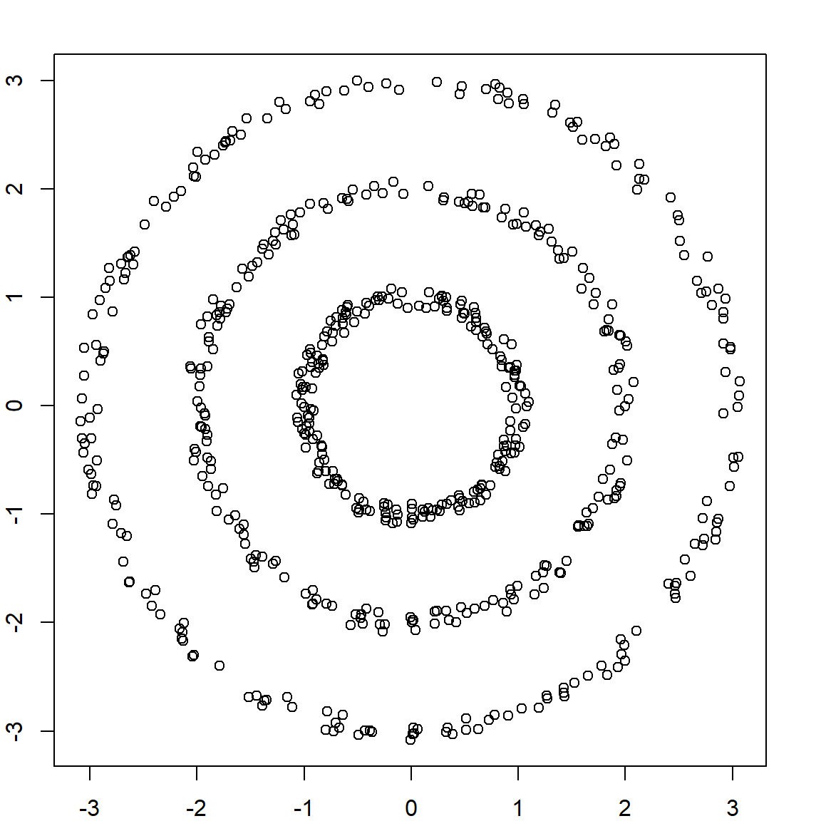
We can perform UMAP using the default tuning. This will create a two-dimensional embedding.
  library(umap)
  circles.umap = umap(X)
  circles.umap
## umap embedding of 600 items in 2 dimensions
## object components: layout, data, knn, config

  plot(circles.umap$layout, col = circle.labels)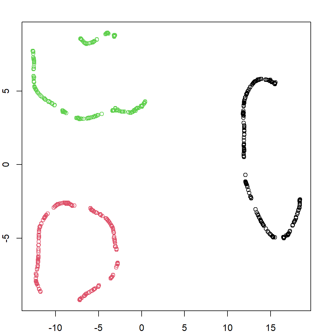
We can see that UMAP learns these new features, which groups similar observations together. Its reasonable to expect that if we perform any clustering algorithm on these new embedded features, we will recover the truth.
29.2 Tuning
UMAP involves a lot of tuning parameters and the most significant one concerns about how we create the (KNN) graph in the first step. You can see the summary of all tuning parameters:
  umap.defaults
## umap configuration parameters
##            n_neighbors: 15
##           n_components: 2
##                 metric: euclidean
##               n_epochs: 200
##                  input: data
##                   init: spectral
##               min_dist: 0.1
##       set_op_mix_ratio: 1
##     local_connectivity: 1
##              bandwidth: 1
##                  alpha: 1
##                  gamma: 1
##   negative_sample_rate: 5
##                      a: NA
##                      b: NA
##                 spread: 1
##           random_state: NA
##        transform_state: NA
##                    knn: NA
##            knn_repeats: 1
##                verbose: FALSE
##        umap_learn_args: NA
To change the default value, we can do the following
myumap.tuning = umap.defaults
umap.defaults$n_neighbors = 5
circles.umap = umap(X, umap.defaults)
plot(circles.umap$layout, col = circle.labels)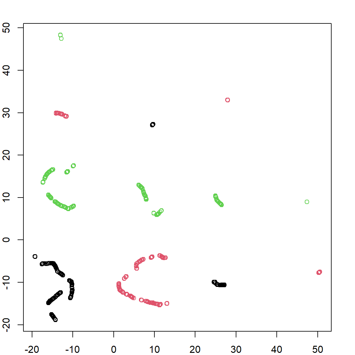 You can see that the result is not as perfect as we wanted. It seems that there are more groups, although each group only involves one type of data. There are other parameter you may consider tuning. For example
 n_components controls how many dimensions you reduced data should have. Usually we don’t use values larger than three, but this is very problem specific.
29.3 Another Example
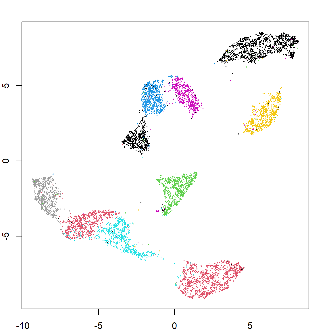
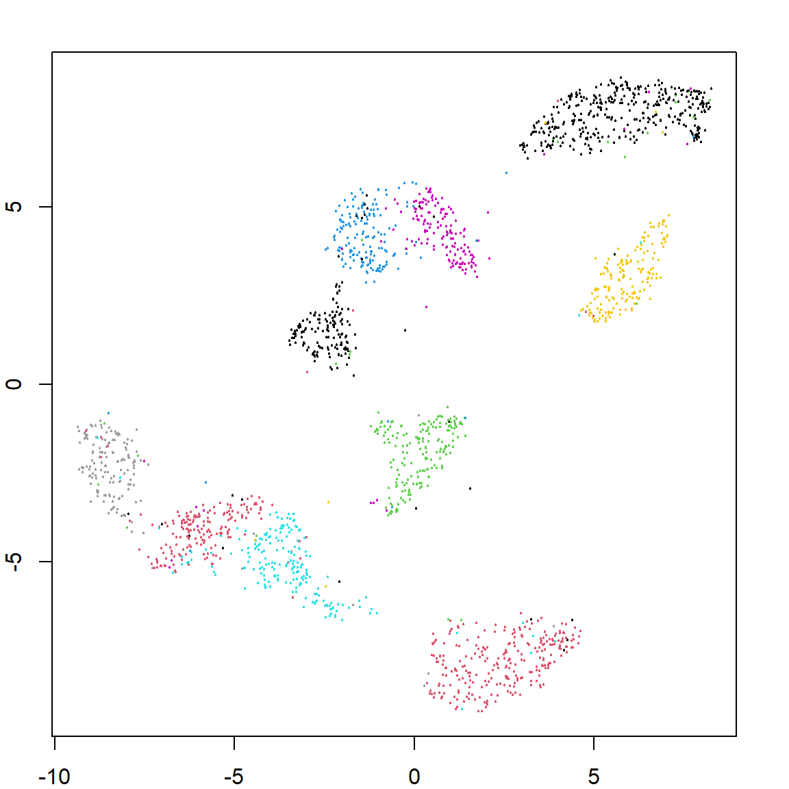
Let’s use UMAP on a larger data, the hand written digit data. We will perform clustering on just the pixels. We can also predict the embedding feature values for future observations. We can see that both recovers the true labels pretty well.
  library(ElemStatLearn)
  dim(zip.train)
## [1] 7291  257
  dim(zip.test)
## [1] 2007  257

  zip.umap = umap(zip.train[, -1])
  zip.pred = predict(zip.umap, zip.test[, -1])

  plot(zip.umap$layout, col = zip.train[, 1]+1, pch = 19, cex = 0.2)