Chapter 28 Spectral Clustering
Spectral clustering aims at clustering observations based on their proximity information. It essentially consists of two steps. The first step is a feature embedding, or dimension reduction. We first construct the graph Laplacian \(\mathbf{L}\) (or normalized version), which represent the proximity information, and perform eigen-decomposition of the matrix. This allows us to use a lower dimensional matrix to represent the proximity information of the original data. Once we have the low-dimensional data, we can perform the regular clustering algorithm, i.e., \(k\)-means on the new dataset.
28.1 An Example
Let’s look at an example that regular \(k\)-means would fail.
  set.seed(1)

  n = 200

  r = c(rep(1, n), rep(2, n), rep(3, n)) + runif(n*3, -0.1, 0.1)
  theta = runif(n) * 2 * pi

  x1 = r * cos(theta)
  x2 = r * sin(theta)
  X = cbind(x1, x2)

  plot(X)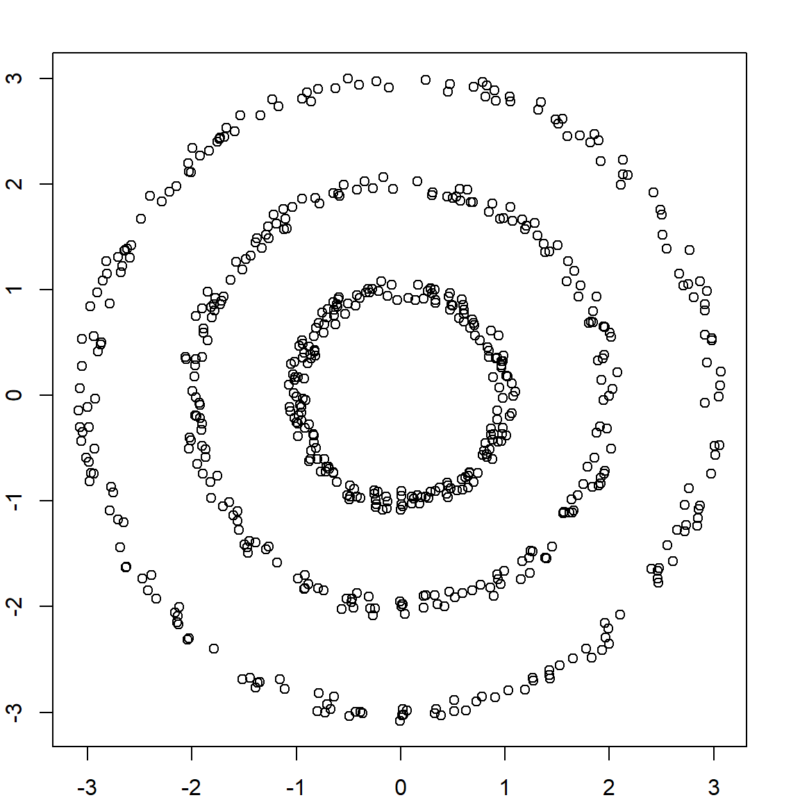
Since \(k\)-means use Euclidean distance, it is not appropriate for such problems.
28.2 Adjacency Matrix
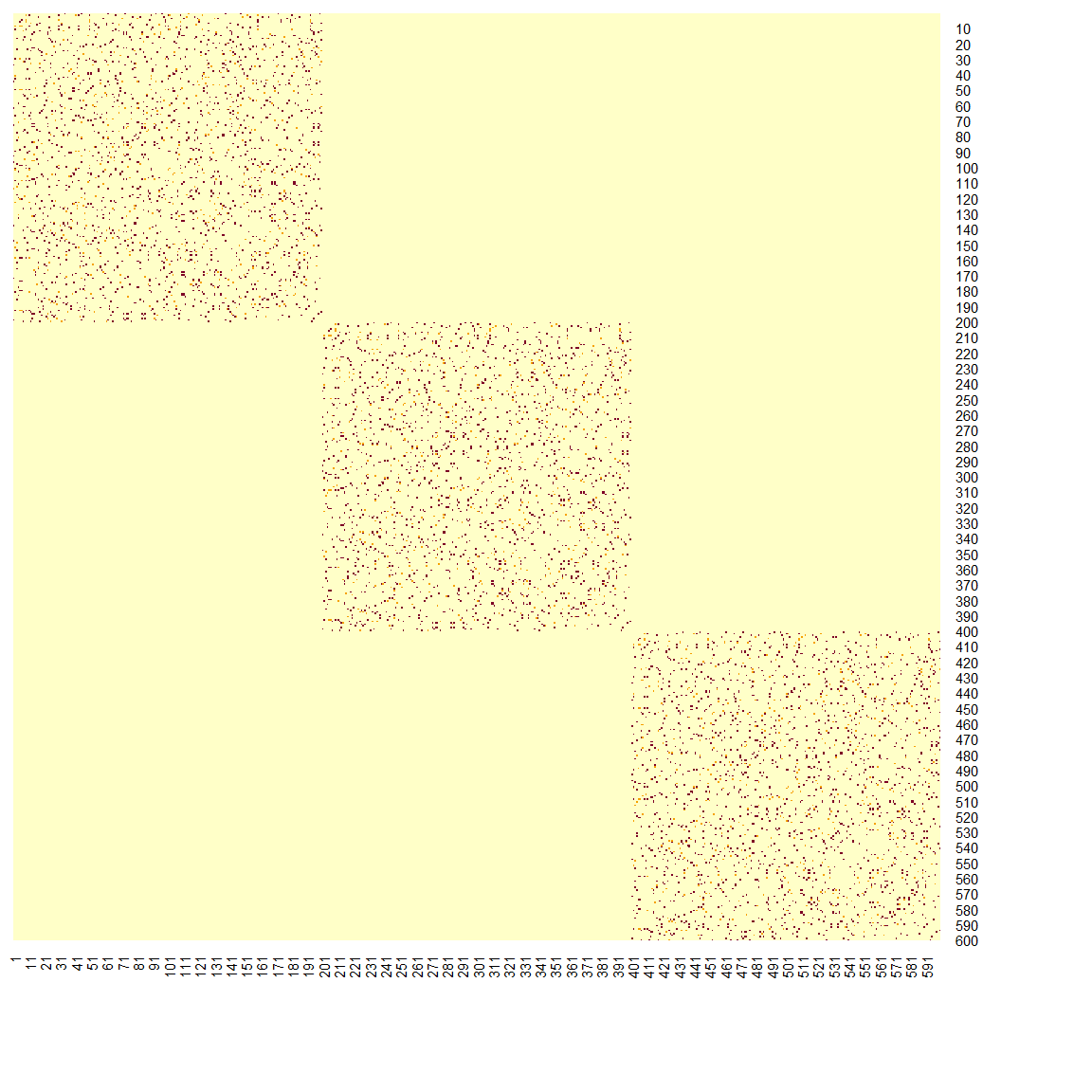
Maybe we should use a nonlinear way to describe the distance/closeness between subjects. For example, let’s define two sample to be close if they are within the k-nearest neighbors of each other. We use \(k = 10\), and create an adjacency matrix \(\mathbf{W}\).
  library(FNN)
##
## Attaching package: 'FNN'
## The following objects are masked from 'package:class':
##
##     knn, knn.cv

  W = matrix(0, 3*n, 3*n)

  # get neighbor index for each observation
  nn = get.knn(X, k=10)

  # write into W
  for (i in 1:(3*n))
    W[i, nn$nn.index[i, ]] = 1

  # W is not necessary symmetric
  W = 0.5*(W + t(W))
  # we may also use
  # W = pmax(W, t(W))
Let’s use a heatmap to display what the adjacency information look like. Please note that our data are ordered with clusters 1, 2 and 3.
28.3 Laplacian Matrix
The next step is to calculate the Laplacian
\[\mathbf{L} = \mathbf{D} - \mathbf{W},\] where \(\mathbf{D}\) is a diagonal matrix with its elements equation to the row sums (or column sums) of \(\mathbf{W}\). We will then perform eigen-decomposition on \(\mathbf{L}\) to extract/define some underlying features.
28.4 Derivation of the Feature Embedding
Assuming that we want to create artificial embedded features that reflects the underlying structure of the data, especially the graph structure. This can be done through an eigen-decomposition of the Laplacian matrix. To see this, let’s assume that the new artificial embedded feature would assign a value \(f_i\) to each observation \(i\). Hence, we want \(f_i\) to be close to \(f_j\) if \(i\) and \(j\) are close in the graph, i.e., when \(w_{ij}\) is large. This can be achieved by
\[\underset{f}{\min} \sum_{i,j} w_{ij} (f_i - f_j)^2.\] To solve this problem, we start with the following matrix form
\[\begin{align*} f^\text{T}\mathbf{L} f &= f^\text{T}\mathbf{D} f - f^\text{T}\mathbf{W} f \\ &= \sum_{i} d_{i} f_i^2 - \sum_{i,j} w_{ij} f_i f_j \\ &= \frac{1}{2} \bigg\{ \sum_{ij} w_{ij} f_i^2 - 2 \sum_{i,j} \mathbf{w}_{ij} f_i f_j + \sum_{ij} w_{ij} f_j^2 \bigg\}\\ &= \frac{1}{2} \sum_{ij} w_{ij} (f_i - f_j)^2. \end{align*}\]
Hence, finding the embedded feature simply becomes an eigen-decomposition problem, i.e., getting the smallest eigen-values of \(\mathbf{L}\). However, it should be noted that when all \(f_i\)’s are identical, \(f^\text{T}\mathbf{L} f\) would be zero. Hence, we should be using the second smallest eigen-values.
  # eigen-decomposition
  f = eigen(L, symmetric = TRUE)

  # plot the smallest eigen-values
  # there are three zero eigen-values, why?
  plot(rev(f$values)[1:10], pch = 19, ylab = "eigen-values",
       col = c(rep("red", 3), rep("blue", 17)))
28.5 Feature Embedding
In fact the smallest eigen-value will always be zero. However, we can use the eigen-vectors associated with the second and third smallest eigen-values. They define some feature embedding or dimension reduction to represent the original data. Since we know the underlying model, two dimensions are enough (to separate three clusters). However, based on the eigen-value plot, there is a big gap between the third and the fourth one. Hence, we only need three. Further removing the smallest one, only two are needed.
  par(mfrow=c(1,2))
  plot(f$vectors[, length(f$values)-1], type = "l", ylab = "eigen-values", ylim = c(-0.1, 0.1))
  plot(f$vectors[, length(f$values)-2], type = "l", ylab = "eigen-values", ylim = c(-0.1, 0.1))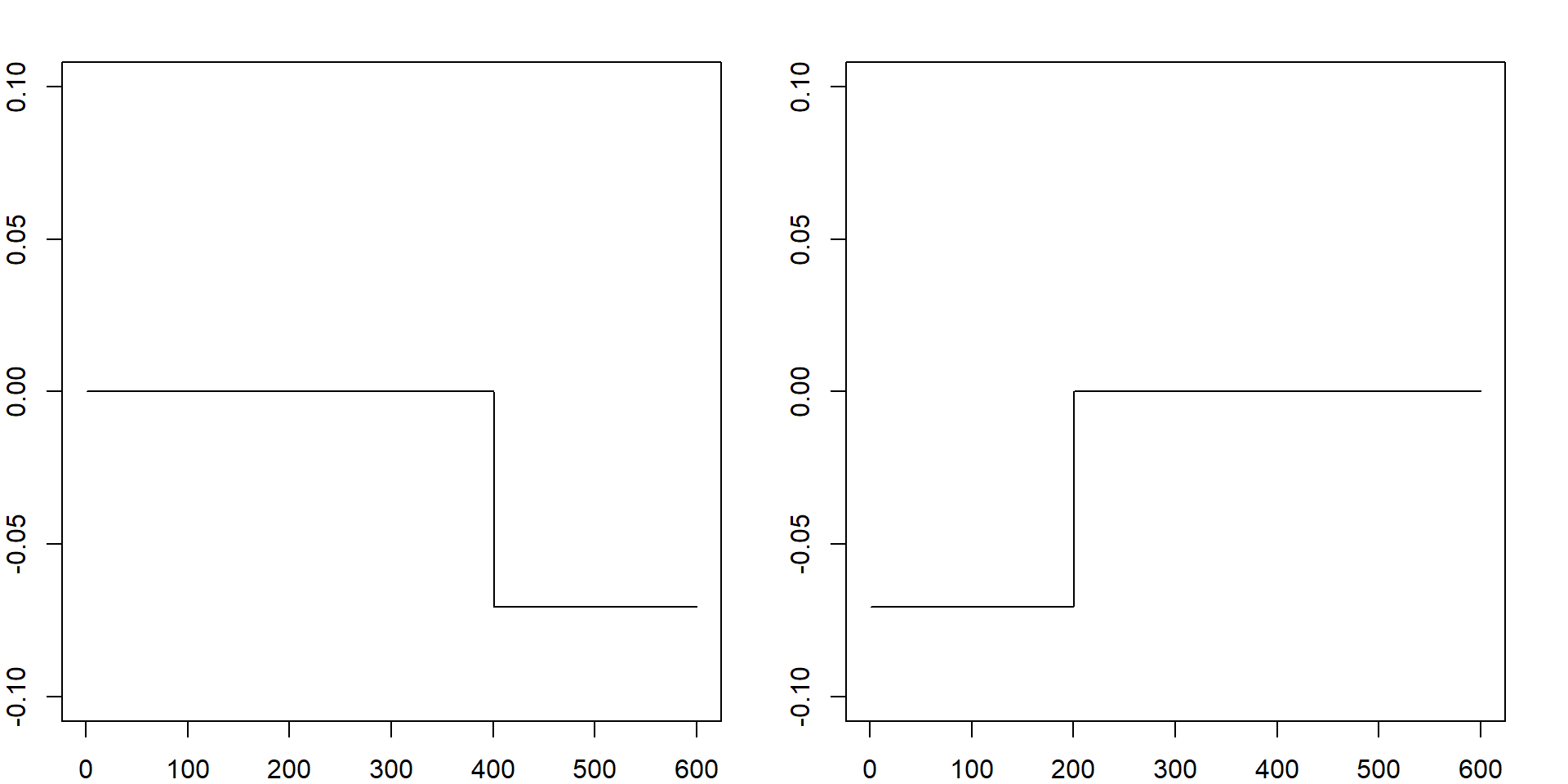
28.6 Clustering with Embedded Features
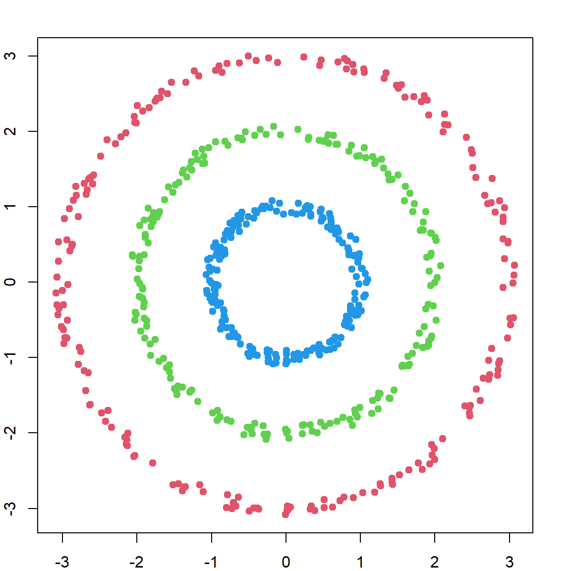
We can then perform \(k\)-means on these two new features. And it will give us the correct clustering.
par(mfrow=c(1,1))
scfit = kmeans(f$vectors[, (length(f$values)-2) : (length(f$values)-1) ], centers = 3, nstart = 20)
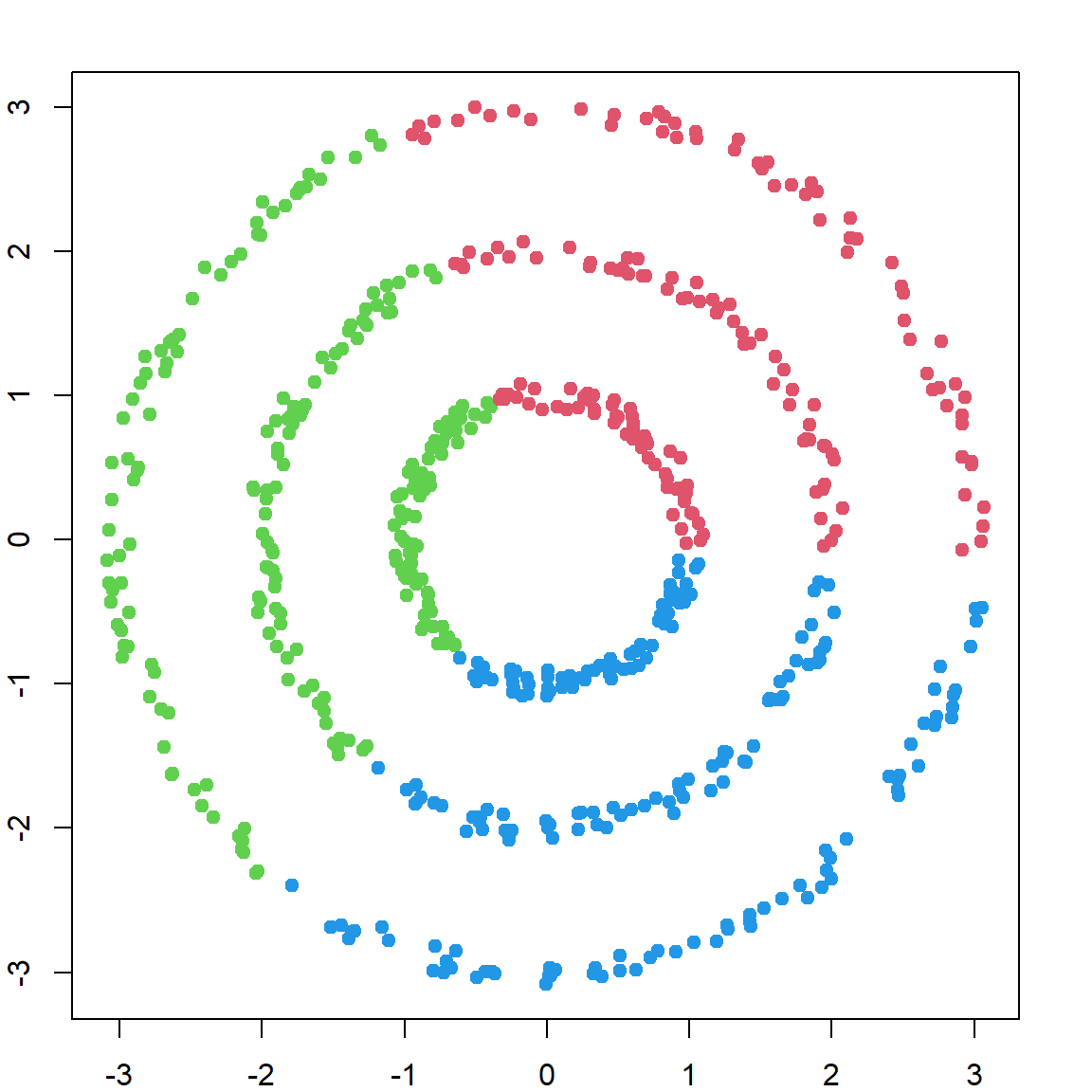
plot(X, col = scfit$cluster + 1, pch = 19)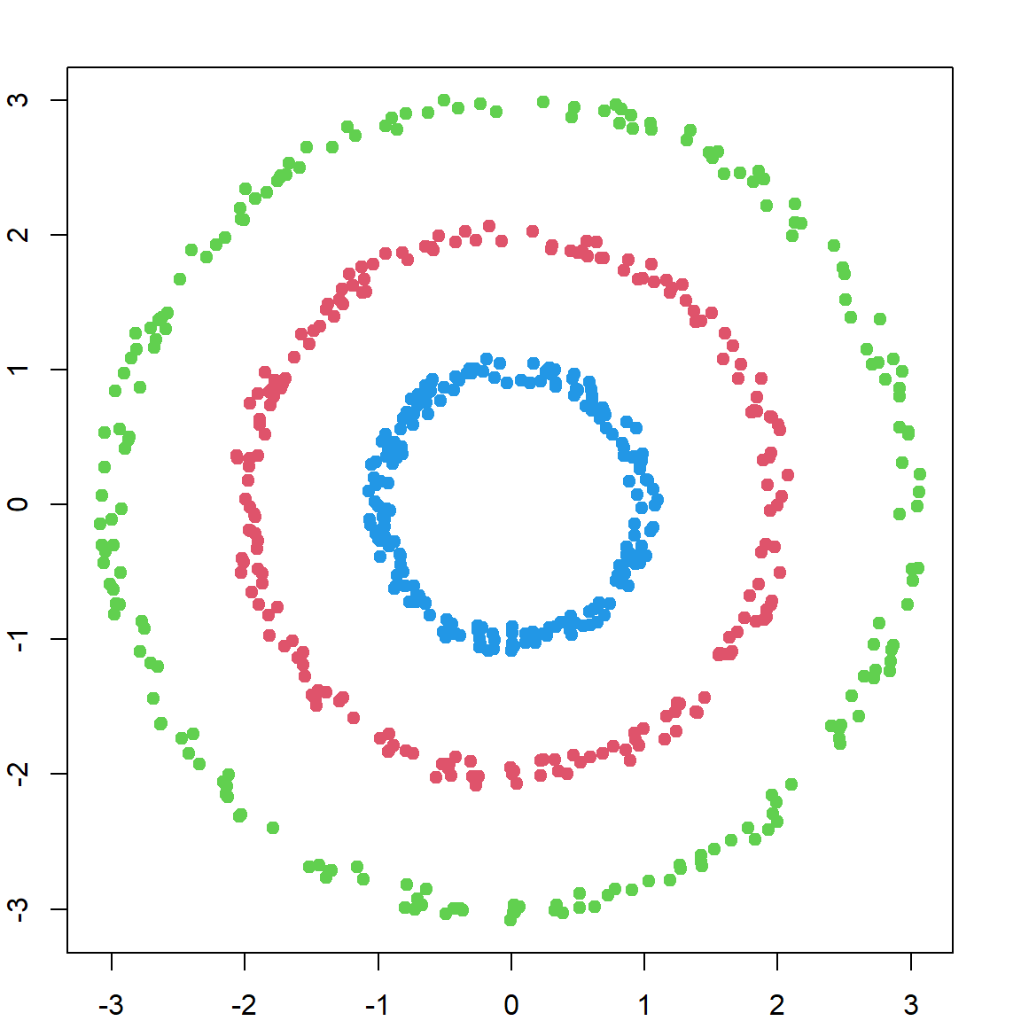
28.7 Normalized Graph Laplacian
There are other choices of the Laplacian matrix. For example, a normalized graph Laplacian is defined as \[\mathbf{L}_\text{sym} = \mathbf{I} - \mathbf{D^{-1/2} \mathbf{W} D^{-1/2}}\]
For our problem, it achieves pretty much the same effect.
  # the normed laplacian matrix
  L = diag(nrow(W)) - diag(1/sqrt(d)) %*% W %*% diag(1/sqrt(d))

  # eigen-decomposition
  f = eigen(L, symmetric = TRUE)

  # perform clustering
  scfit = kmeans(f$vectors[, (length(f$values)-2) : (length(f$values)-1) ], centers = 3, nstart = 20)
  plot(X, col = scfit$cluster + 1, pch = 19)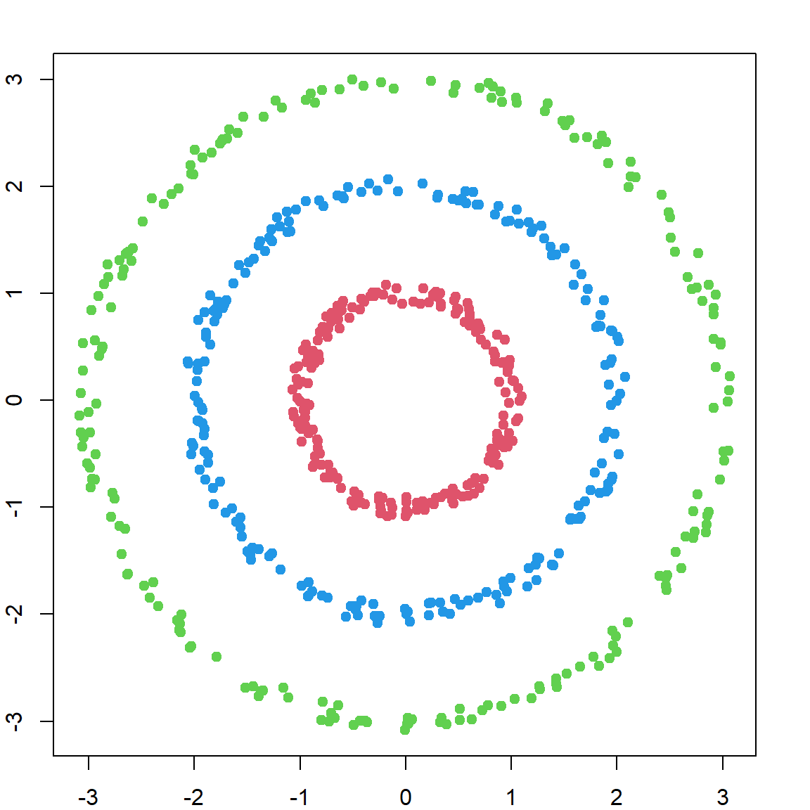
28.8 Using a Different Adjacency Matrix
Let’s also try to use the Gaussian kernel to define the adjacency matrix. Here, tuning (the bandwidth parameter in the kernel function) becomes important for the performance.
  # the Gaussian kernel
  W = exp(-as.matrix(dist(X/0.2))^2)

  # view the adjacency matrix
  heatmap(W, Rowv = NA, Colv=NA, symm = TRUE, revC = TRUE)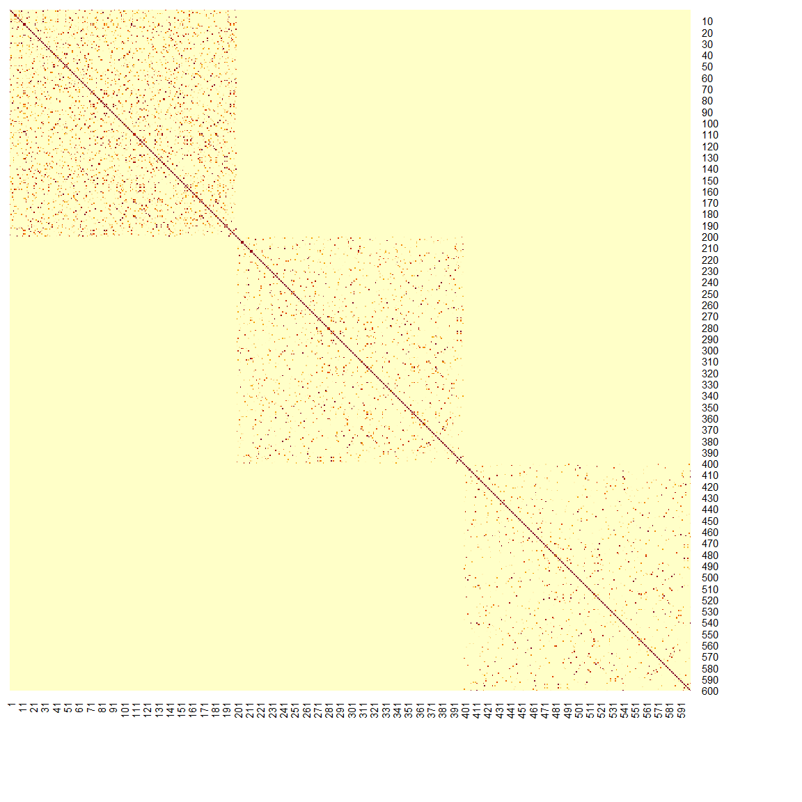
  # the normed laplacian matrix
  L = diag(colSums(W)) - W

  # eigen-decomposition
  f = eigen(L, symmetric = TRUE)

  # perform clustering
  scfit = kmeans(f$vectors[, (length(f$values)-2) : (length(f$values)-1) ], centers = 3, nstart = 20)
  plot(X, col = scfit$cluster + 1, pch = 19)