Chapter 25 Hierarchical Clustering
25.1 Basic Concepts
Suppose we have a set of six observations:

The goal is to progressively group them together until there is only one group. During this process, we will always choose the closest two groups (some may be individuals) to merge.

If we evaluate the distance between two observations, that would be very easy. For example, the Euclidean distance and Hamming distance can be used. But what about the distance between two groups? Suppose we have two groups of observations \(G\) and \(H\), then several distance metric can be considered:
- Complete linkage: the furthest pair \[d(G, H) = \underset{i \in G, \, j \in G}{\max} d(x_i, x_j)\]
- Single linkage: the closest pair \[d(G, H) = \underset{i \in G, \, j \in G}{\min} d(x_i, x_j)\]
- Average linkage: average distance \[d(G, H) = \frac{1}{n_G n_H} \sum_{i \in G} \sum_{i \in H} d(x_i, x_j)\]
The R function hclust() uses the complete linkage as default. To perform a hierarchical clustering, we need to know all the pair-wise distances, i.e., \(d(x_i, x_j)\). Let’s consider the Euclidean distance.
  # the Euclidean distance can be computed using dist()
  as.matrix(dist(x))
##          1         2         3         4         5         6
## 1 0.000000 1.2294164 1.7864196 1.1971565 1.4246185 1.5698349
## 2 1.229416 0.0000000 2.3996575 0.8727261 1.9243764 2.2708670
## 3 1.786420 2.3996575 0.0000000 2.8586738 0.4782442 0.2448835
## 4 1.197156 0.8727261 2.8586738 0.0000000 2.4219048 2.6741260
## 5 1.424618 1.9243764 0.4782442 2.4219048 0.0000000 0.4204479
## 6 1.569835 2.2708670 0.2448835 2.6741260 0.4204479 0.0000000
We use this distance matrix in the hierarchical clustering algorithm hclust(). The plot() function will display the merging process. This should be exactly the same as we demonstrated previously.
The height of each split represents how separated the two subsets are (the distance when they are merged). Selecting the number of clusters is still a tricky problem. Usually, we pick a cutoff where the height of the next split is short. Hence, the above example fits well with two clusters.
25.2 Example 1: iris data
The iris data contains three clusters and four variables. We use all variables in the distance calculation and use the default complete linkage.

This does not seem to perform very well, considering that we know the true number of classes is three. This shows that, in practice, the detected clusters can heavily depend on the variables you use. Let’s try some other linkage functions.
This looks better, at least more consistent with the truth. Now we can also consider using other package to plot this result. For example, the ape package provides some interesting choices.
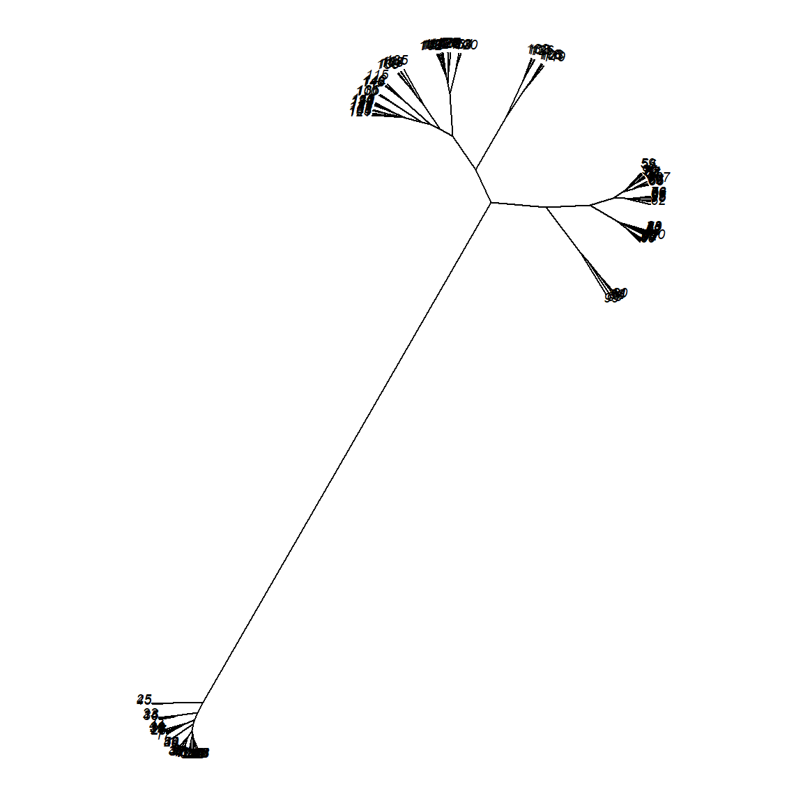
We can also add the true class colors to the plot. This plot is motivated by the dendextend package vignettes. Of course in a realistic situation, we wouldn’t know what the true class is.
25.3 Example 2: RNA Expression Data
We use a tissue gene expression dataset from the tissuesGeneExpression library, available from bioconductor. I prepared the data to include only 100 genes. You can download the data from the course website. In this first step, we simply plot the data using a heatmap. By default, a heatmap uses red to denote higher values, and yellow for lower values. Note that we first plot the data without organizing the columns or rows. The data is also standardized based on columns (genes).
    load("data/tissue.Rda")
    dim(expression)
## [1] 189 100
    table(tissue)
## tissue
##  cerebellum       colon endometrium hippocampus      kidney       liver    placenta
##          38          34          15          31          39          26           6
    head(expression[, 1:3])
##                 211298_s_at 203540_at 211357_s_at
## GSM11805.CEL.gz    7.710426  5.856596   12.618471
## GSM11814.CEL.gz    4.741010  5.813841    5.116707
## GSM11823.CEL.gz   11.730652  5.986338   13.206078
## GSM11830.CEL.gz    5.061337  6.316815    9.780614
## GSM12067.CEL.gz    4.955245  6.561705    8.589003
## GSM12075.CEL.gz   10.469501  5.880740   13.050554
    heatmap(scale(expression), Rowv = NA, Colv = NA)
Hierarchical clustering may help us discover interesting patterns. If we reorganize the columns and rows based on the clusters, then it may reveal underlying subclasses of issues, or subgroups of genes.
Note that there are many other R packages that produce more interesting plots. For example, you can try the heatmaply package.