Chapter 27 Self-Organizing Map
27.1 Basic Concepts
I found the best demonstration of the Self-Organizing Map algorithm is the following graph that displays it over iterations. It is available at this website:
Let’s understand this by pairing it with the algorithm. There are several different algorithms available, but one of the most popular ones is proposed by Kohonen (1990). Here, we present a SOM with a 2-dimensional output. The following are the inputs:
- \(\{x_i\}_{i=1}^n\) is a set of \(n\) observations, with dimension \(p\) (the yellow and green dots in the figure).
- \(w_{ij}\), \(i = 1, \ldots p\), \(j = 1, \ldots q\) are a grid of centers (the connected black dots). They are similar to the centers in a k-mean algorithm. However, they also preserve some geometric relationships among \(w_{ij}\)’s, meaning that \(w_{ij}\)’s are closer if their indices \({i, j}\) are closer (connected in the figure).
- \(\alpha\) this is a learning rate between \([0, 1]\). This controls how fast the \(w_{ij}\)’s are updated.
- \(r\) is also a tuning parameter. This controls how many \(w_{ij}\)’s will be updated at each iteration
Now, we look at the algorithm. This is different from \(k\)-means because we do not use all the observations immediately. The algorithm works by stream-in the observations one-by-one. Whenever a new observation \(x_k\), \(k = 1, \ldots, n\) comes in, we will update the centers \(w_{ij}\)’s by the following:
- For all \(w_{ij}\), calculate the distance between each \(w_{ij}\) and \(x_k\). Let \(d_{ij} = \lVert x_k - w_{ij} \rVert\). By default, we use Euclidean distance.
- Select the closest \(w_{ij}\), denoted as \(w_{\ast}\)
- Update each \(w_{ij}\) based on the fomular \(w_{ij} = w_{ij} + \alpha \, h(w_\ast, w_{ij}, r) \, \lVert x_k - w_{ij} \rVert\)
After each iteration (updating with one more observation), we will decrease the value of \(\alpha\) and \(r\). In the kohonen package, the \(\alpha\) starts at 0.05, and gradually decreases to 0.01, while \(r\) is chosen to be 2/3 of all cluster means at the first iteration.
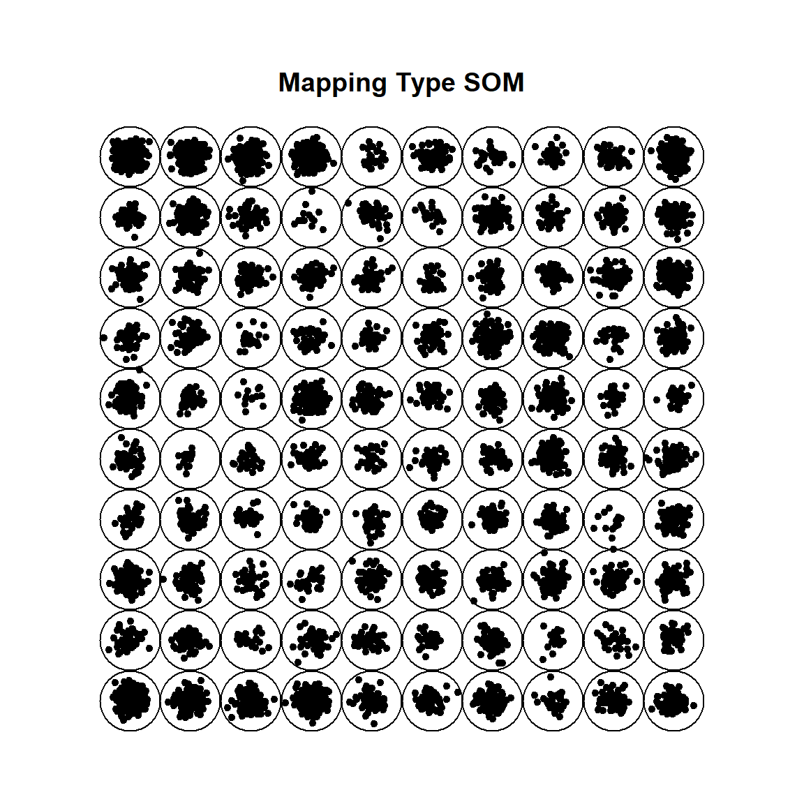
Using the kohonen package, we perform a SOM on the Handwritten Digit Recognition Data. The heatmap shows how each \(w_{ij}\) is away from it’s neighboring \(w_{ij}\)’s. The extreme bright one means that the center is quite isolated by itself.
  library(kohonen)
##
## Attaching package: 'kohonen'
## The following object is masked from 'package:class':
##
##     somgrid

  # Handwritten Digit Recognition Data
  library(ElemStatLearn)

  # the first column is the true digit
  dim(zip.train)
## [1] 7291  257

  # for speed concern, I only use a few variables (pixels)
  zip.SOM <- som(zip.train[, seq(2, 257, length.out = 10)],
                 grid = somgrid(10, 10, "rectangular"))
  plot(zip.SOM, type = "dist.neighbours")
  # plot(zip.SOM, main = "Default SOM Plot")

  # you can try using all the pixels
  # zip.SOM <- som(zip.train[, 2:257],
  #            grid = somgrid(10, 10, "rectangular"))
  # plot(zip.SOM, type = "dist.neighbours")
We could also look at the class labels (digits) coming out of the SOM. Particularly the plot on the right-hand side shows the proportion of subjects with each label for the subjects in each cluster (using a pie chart).
    set.seed(1)
    zip.SOM2 <- xyf(zip.train[, seq(2, 257, length.out = 10)],
                    classvec2classmat(zip.train[, 1]),
                    grid = somgrid(10, 10, "hexagonal"), rlen = 300)
    par(mfrow = c(1, 2))
    plot(zip.SOM2, type = "codes", main = c("Codes X", "Codes Y"))
    zip.SOM2.hc <- cutree(hclust(dist(zip.SOM2$codes[[2]])), 10)
    add.cluster.boundaries(zip.SOM2, zip.SOM2.hc)