Chapter 5 Optimization Basics
Optimization is heavily involved in statistics and machine learning. Almost all methods introduced in this book can be viewed as some form of optimization. It would be good to have some prior knowledge of it so that later chapters can use these concepts without difficulties. Especially, one should be familiar with concepts such as constrains, gradient methods, and be able to implement them using existing R functions. Since optimization is such a broad topic, we refer readers to Boyd and Vandenberghe (2004) and Nocedal and Wright (2006) for more further reading.
We will use a slightly different set of notations in this Chapter so that we are consistent with the literature. This means that for the most part, we will use \(x\) as our parameter of interest and optimize a function \(f(x)\). This is in contrast to optimizing \(\theta\) in a statistical model \(f_\theta(x)\) where \(x\) is the observed data. However, in the example of linear regression, we may again switch back to the regular notation of \(x^\text{T} \boldsymbol{\beta}\). These transitions will only happen under clear context and should not create ambiguity.
5.1 Basic Concept
We usually consider a convex optimization problem (non-convex problems are a bit too involving although we will also see some examples of that), meaning that we optimize (minimize) a convex function in a convex domain. A convex function \(f(\mathbf{x})\) maps some subset \(C \in \mathbb{R}^p\) into \(\mathbb{R}^p\), but enjoys the property that
\[ f(t \mathbf{x}_1 + (1 - t) \mathbf{x}_2) \leq t f(\mathbf{x}_1) + ( 1- t) f(\mathbf{x}_2), \] for all \(t \in [0, 1]\) and any two points \(\mathbf{x}_1\), \(\mathbf{x}_2\) in the domain of \(f\).
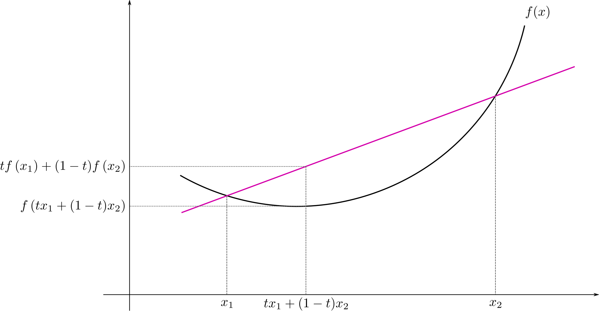
Note that if you have a concave function (the bowl faces downwards) then \(-f(\mathbf{x})\) would be convex. Examples of convex functions:
- Univariate functions: \(x^2\), \(\exp(x)\), \(-log(x)\)
- Affine map: \(a^\text{T}\mathbf{x}+ b\) is both convex and concave
- A quadratic function \(\frac{1}{2}\mathbf{x}^\text{T}\mathbf{A}\mathbf{x}+ b^\text{T}\mathbf{x}+ c\), if \(\mathbf{A}\) is positive semidefinite
- All \(p\) norms are convex, following the Triangle inequality and properties of a norm.
- A sin function is neither convex or concave
On the other hand, a convex set \(C\) means that if we have two points \(x_1\) and \(x_2\) in \(C\), the line segment joining these two points has to lie within \(C\), i.e.,
\[\mathbf{x}_1, \mathbf{x}_2 \in C \quad \Longrightarrow \quad t \mathbf{x}_1 + (1 - t) \mathbf{x}_2 \in C,\] for all \(t \in [0, 1]\).
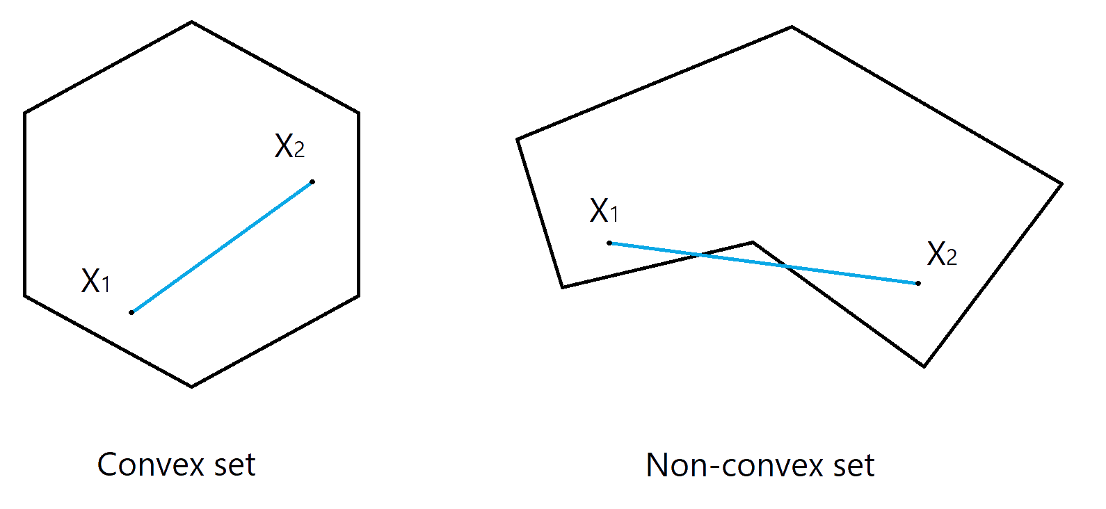
Examples of convex set include
- Real line: \(\mathbb{R}\)
- Norm ball: \(\{ \mathbf{x}: \lVert \mathbf{x}\rVert \leq r \}\)
- Hyperplane: \(\{ \mathbf{x}: a^\text{T}\mathbf{x}= b \}\)
Consider a simple optimization problem:
\[ \text{minimize} \quad f(x_1, x_2) = x_1^2 + x_2^2\]
Clearly, \(f(x_1, x_2)\) is a convex function, and we know that the solution of this problem is \(x_1 = x_2 = 0\). However, the problem might be a bit more complicated if we restrict that in a certain (convex) region, for example,
\[\begin{align} &\underset{x_1, x_2}{\text{minimize}} & \quad f(x_1, x_2) &= x_1^2 + x_2^2 \\ &\text{subject to} & x_1 + x_2 &\leq -1 \\ & & x_1 + x_2 &> -2 \end{align}\]
Here the convex set \(C = \{x_1, x_2 \in \mathbb{R}: x_1 + x_2 \leq -1 \,\, \text{and} \,\, x_1 + x_2 > -2\}\). And our problem looks like the following, which attains it minimum at \((-0.5, -0.5)\).
In general, we will be dealing with a problem in the form of
\[\begin{align} &\underset{\mathbf{x}}{\text{minimize}} & \quad f(\mathbf{x}) \\ &\text{subject to} & g_i(\mathbf{x}) & \leq 0, \, i = 1,\ldots, m \\ & & h_j(\mathbf{x}) &= 0, \, j = 1,\ldots, k \end{align}\]
where \(g_i(\mathbf{x})\)s are a set of inequality constrains, and \(h_j(\mathbf{x})\)s are equality constrains. There are established result showing what type of constrains would lead to a convex set, but let’s assuming for now that we will be dealing a well behaved problem. We shall see in later chapters that many models such as, Lasso, Ridge and support vector machines can all be formulated into this form.
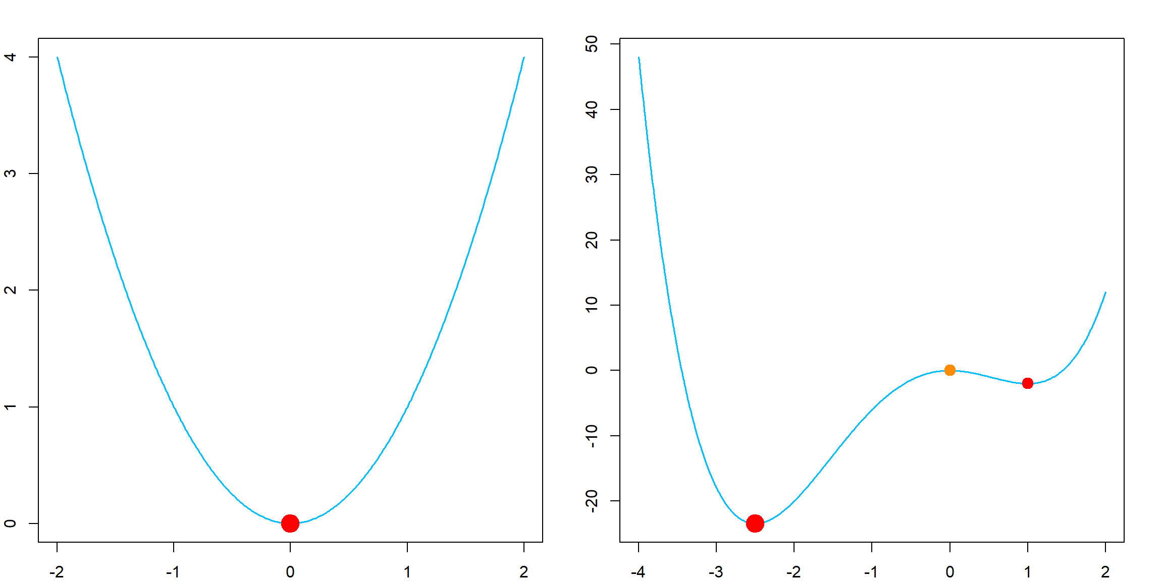
5.2 Global vs. Local Optima
Although we would like to deal with convex optimization problems, non-convex problems appears more and more frequently. For example, deep learning models are almost always non-convex except overly simplified ones. However, for convex optimization problems, a local minimum is also a global minimum, i.e., a \(x^\ast\) such that for any \(x\) in the feasible set, \(f(x^\ast) \leq f(x)\). This can be achieved by a variety of descent algorithms, to be introduced. However, for non-convex problems, we may still be interested in a local minimum, which satisfies that for any \(x\) in a neighboring set of \(x^\ast\), \(f(x^\ast) \leq f(x)\). The comparison of these two cases can be demonstrated in the following plots. Again, a descent algorithm can help us find a local minimum, except for some very special cases, such as a saddle point. However, we will not discuss these issues in this book.
5.3 Example: Linear Regression using optim()
Although completely not necessary, we may also view linear regression as an optimization problem. This is of course an unconstrained problem, meaning that \(C \in \mathbb{R}^p\). Such problems can be solved using the optim() function. Also, let’s temporarily switch back to the \(\boldsymbol{\beta}\) notation of parameters. Hence, if we observe a set of observations \(\{\mathbf{x}_i, y_i\}_{i = 1}^n\), our optimization problem is to minimize the objection function, i.e., residual sum of squares (RSS):
\[\begin{align} \underset{\boldsymbol{\beta}}{\text{minimize}} \quad f(\boldsymbol{\beta}) = \frac{1}{n} \sum_i (y_i - \mathbf{x}_i^\text{T}\boldsymbol{\beta})^2 \\ \end{align}\]
We generate 200 random observations, and also write a function to calculate the RSS for any given \(\boldsymbol{\beta}\) values. The objective function looks like the following:
    # generate data from a simple linear model
    set.seed(20)
    n = 200
    x <- cbind(1, rnorm(n))
    y <- x %*% c(0.5, 1) + rnorm(n)

    # calculate the residual sum of squares for a grid of beta values
    rss <- function(b, trainx, trainy) sum((trainy - trainx %*% b)^2)
Now the question is how to solve this problem. The optim() function uses the following syntax:
    # The solution can be solved by any optimization algorithm
lm.optim <- optim(par = c(2, 2), fn = rss, trainx = x, trainy = y)- The
parargument specifies an initial value, in this case, \(\beta_0 = \beta_1 = 2\) - The
fnargument specifies the name of anRfunction that can calculate the objective function. Please note that the first argument in this function has be the parameter being optimized, i.e, \(\boldsymbol{\beta}\). Also, it must be a vector, not a matrix or other types. - The arguments
trainx = x,trainy = yspecifies any additional arguments that the objective functionfn, i.e.,rssneeds. It behaves the same as if you are supplying this torss.
    lm.optim
## $par
## [1] 0.4532072 0.9236502
##
## $value
## [1] 203.5623
##
## $counts
## function gradient
##       63       NA
##
## $convergence
## [1] 0
##
## $message
## NULL
The result shows that the estimated parameters ($par) are 0.453 and 0.924, with a functional value 203.562. The convergence code is 0, meaning that the algorithm converged. The parameter estimates are almost the same as lm(), with small numerical errors.
    # The solution form lm()
    summary(lm(y ~ x - 1))$coefficients
##     Estimate Std. Error   t value     Pr(>|t|)
## x1 0.4530498 0.07177854  6.311772 1.773276e-09
## x2 0.9236934 0.07226742 12.781602 1.136397e-27
What we will be introducing in the following are some basic approaches to solve such a numerical problem. We will start with unconstrained problems, then introduce constrained problems.
5.4 First and Second Order Properties
These properties are usually applied to unconstrained optimization problems. They are essentially just describing the landscape around a point \(\mathbf{x}^\ast\) such that it becomes the local optimizer. Since we generally concerns a convex problem, a local solution is also the global solution. However, these properties are still generally applied when solving a non-convex problem. Note that these statements are multi-dimensional.
First-Order Necessary Conditions: If \(f\) is continuously differentiable in an open neighborhood of local minimum \(\mathbf{x}^\ast\), then \(\nabla f(\mathbf{x}^\ast) = \mathbf{0}\).
When we have a point \(\mathbf{x}^\ast\) with \(\nabla f(\mathbf{x}^\ast) = \mathbf{0}\), we call \(\mathbf{x}^\ast\) a stationary point. This is only a necessary condition, but not sufficient. Since example, \(f(x) = x^3\) has zero derivative at \(x = 0\), but this is not an optimizer. The figure in @ref(global_local) also contains such a point. TO further strengthen this, we have
Second-order Necessary Conditions: If \(f\) is twice continuously differentiable in an open neighborhood of local minimum \(\mathbf{x}^\ast\), then \(\nabla f(\mathbf{x}^\ast) = \mathbf{0}\) and \(\nabla^2 f(\mathbf{x}^\ast)\) is positive semi-definite.
This does rule out some cases, with a higher cost (\(f\) needs to be twice continuously differentiable). But requiring positive semi-definite would not ensure everything. The same example \(f(x) = x^3\) still satisfies this, but its not a local minimum. A positive definite \(\nabla^2 f(\mathbf{x}^\ast)\) would be sufficient:
Second-order Sufficient Conditions: \(f\) is twice continuously differentiable in an open neighborhood of \(\mathbf{x}^\ast\). If \(\nabla f(\mathbf{x}^\ast) = \mathbf{0}\) and \(\nabla^2 f(\mathbf{x}^\ast)\) is positive definite, i.e., \[ \nabla^2 f(\mathbf{x}) = \left(\frac{\partial^2 f(\mathbf{x})}{\partial x_i \partial x_j}\right) = \mathbf{H}(\mathbf{x}) \succ 0 \]
then \(\mathbf{x}^\ast\) is a strict local minimizer of \(f\). Here \(\mathbf{H}(\mathbf{x})\) is called the Hessian matrix, which will be frequently used in second-order methods.
5.5 Algorithm
Most optimization algorithms follow the same idea: starting from a point \(\mathbf{x}^{(0)}\) (which is usually specified by the user) and move to a new point \(\mathbf{x}^{(1)}\) that improves the objective function value. Repeatedly performing this to get a sequence of points \(\mathbf{x}^{(0)}, \mathbf{x}^{(1)}, \ldots\) until the certain stopping criterion is reached.
A stopping criterion could be
- Using the gradient of the objective function: \(\lVert \nabla f(\mathbf{x}^{(k)}) \rVert < \epsilon\)
- Using the (relative) change of distance: \(\lVert \mathbf{x}^{(k)} - \mathbf{x}^{(k-1)} \rVert / \lVert \mathbf{x}^{(k-1)}\rVert< \epsilon\) or \(\lVert \mathbf{x}^{(k)} - \mathbf{x}^{(k-1)} \rVert < \epsilon\)
- Using the (relative) change of functional value: \(| f(\mathbf{x}^{(k)}) - f(\mathbf{x}^{(k-1)})| < \epsilon\) or \(| f(\mathbf{x}^{(k)}) - f(\mathbf{x}^{(k-1)})| / |f(\mathbf{x}^{(k)})| < \epsilon\)
- Stop at a pre-specified number of iterations.
Most algorithms differ in terms of how to move from the current point \(\mathbf{x}^{(k)}\) to the next, better target point \(\mathbf{x}^{(k+1)}\). This may depend on the smoothness or structure of \(f\), constrains on the domain, computational complexity, memory limitation, and many others.
5.6 Second-order Methods
5.6.1 Newton’s Method
Now, let’s discuss several specific methods. One of the oldest one is Newton’s method. This is motivated form a quadratic approximation (essentially Taylor expansion) at a current point \(\mathbf{x}\),
\[f(\mathbf{x}^\ast) \approx f(\mathbf{x}) + \nabla f(\mathbf{x})^\text{T}(\mathbf{x}^\ast - \mathbf{x}) + \frac{1}{2} (\mathbf{x}^\ast - \mathbf{x})^\text{T}\mathbf{H}(\mathbf{x}) (\mathbf{x}^\ast - \mathbf{x})\] Our goal is to find a new stationary point \(\mathbf{x}^\ast\) such that \(\nabla f(\mathbf{x}^\ast) = 0\). By taking derivative of the above equation on both sides, with respect to \(\mathbf{x}^\ast\), we need
\[0 = \nabla f(\mathbf{x}^\ast) = 0 + \nabla f(\mathbf{x}) + \mathbf{H}(\mathbf{x}) (\mathbf{x}^\ast - \mathbf{x}) \] which leads to
\[\mathbf{x}^\ast = \mathbf{x}- \mathbf{H}(\mathbf{x})^{-1} \nabla f(\mathbf{x}).\]
Hence, if we are currently at a point \(\mathbf{x}^{(k)}\), we need to calculate the gradient \(\nabla f(\mathbf{x}^{(k)})\) and Hessian \(\mathbf{H}(\mathbf{x})\) at this point, then move to the new point using \(\mathbf{x}^{(k+1)} = \mathbf{x}^{(k)} - \mathbf{H}(\mathbf{x}^{(k)})^{-1} \nabla f(\mathbf{x}^{(k)})\). Some properties and things to concern regarding Newton’s method:
- Newton’s method is scale invariant, meaning that you do not need to worry about the step size. It is automatically taken care of by the Hessian matrix. However, in practice, the local approximation may not be accurate, which makes the new point \(\mathbf{x}^{(k+1)}\) behaves differently than what we expect. Hence, it might still be safe to introduce a smaller step size \(\delta \in (0, 1)\) and move with
\[\mathbf{x}^{(k+1)} = \mathbf{x}^{(k)} - \delta \, \mathbf{H}(\mathbf{x}^{(k)})^{-1} \nabla f(\mathbf{x}^{(k)})\] - There are also alternatives to take care of the step size. For example, line search is frequently used, which will try to find the optimal \(\delta\) that minimizes the function \[f(\mathbf{x}^{(k)} + \delta \mathbf{v})\] where the direction \(\mathbf{v}\) in this case is \(\mathbf{v}= \mathbf{H}(\mathbf{x}^{(k)})^{-1} \nabla f(\mathbf{x}^{(k)})\). It is also popular to use backtracking line search, which reduces the computational cost. The idea is to start with a large \(\delta\) and gradually reduces it by a certain proportion if the new point doesn’t significantly improves, i.e., \[f(\mathbf{x}^{(k)} + \delta \mathbf{v}) > f(\mathbf{x}^{(k)}) - \frac{1}{2} \delta \nabla f(\mathbf{x}^{(k)})^\text{T}\mathbf{v}\] Note that when the direction \(\mathbf{v}\) is \(\mathbf{H}(\mathbf{x}^{(k)})^{-1} \nabla f(\mathbf{x}^{(k)})\), \(\nabla f(\mathbf{x}^{(k)})^\text{T}\mathbf{v}\) is essentially the norm defined by the Hessian matrix.
- When you do not have the explicit formula of Hessian and even the gradient, you may numerically approximate the derivative using the definition. For example, we could use \[ \frac{f(\mathbf{x}^{(k)} + \epsilon) - f(\mathbf{x}^{(k)})}{\epsilon} \] with \(\epsilon\) small enough, e.g., \(10^{-5}\). However, this is very costly for the Hessian matrix if the number of variables is large.
5.6.2 Quasi-Newton Methods
Since the idea of Newton’s method is to solve a vector \(\mathbf{v}\) such that
\[\mathbf{H}(\mathbf{x}^{(k)}) \mathbf{v}= - \nabla f(\mathbf{x}^{(k)}), \] If \(\mathbf{H}\) is difficult to compute, we may use some matrix to substitute it. For example, if we simplify use the identity matrix \(\mathbf{I}\), then this reduces to a first-order method to be introduced later. However, if we can get a good approximation, we can still solve this linear system and get to a better point. Then the question is how to obtain such matrix in a computationally inexpensive way. The Broyden–Fletcher–Goldfarb–Shanno (BFSG) algorithm is such an approach by iteratively updating its (inverse) estimation. The algorithm proceed as follows:
- Start with \(x^{(0)}\) and a positive definite matrix, e.g., \(\mathbf{B}^{(0)} = \mathbf{I}\)
- For \(k = 0, 1, 2, \ldots\),
- Search a updating direction by solving the linear system \(\mathbf{B}^{(k)} \mathbf{p}_k = - \nabla f(\mathbf{x}^{(k)})\)
- Perform line search in the direction of \(\mathbf{v}_k\) and obtain the next point \(\mathbf{x}^{(k+1)} = \mathbf{x}^{(k)} + \delta \mathbf{p}_k\)
- Update the approximation by \[ \mathbf{B}^{(k+1)} = \mathbf{B}^{(k)} + \frac{\mathbf{y}_k^\text{T}\mathbf{y}_{k}}{ \mathbf{y}_{k}^\text{T}\mathbf{s}_{k} } - \frac{\mathbf{B}^{(k)}\mathbf{s}_{k}\mathbf{s}_{k}^\text{T}{\mathbf{B}^{(k)}}^\text{T}}{\mathbf{s}_{k}^\text{T}\mathbf{B}^{(k)} \mathbf{s}_{k} }, \] where \(\mathbf{y}_k = \nabla f(\mathbf{x}^{(k+1)}) - \nabla f(\mathbf{x}^{(k)})\) and \(\mathbf{s}_{k} = \mathbf{x}^{(k+1)} - \mathbf{x}^{(k)}\).
The BFGS is performing a rank-two update by assuming that \[ \mathbf{B}^{(k+1)} = \mathbf{B}^{(k)} + a \mathbf{u}\mathbf{u}^\text{T}+ b \mathbf{v}\mathbf{v}^\text{T},\] Alternatives of such type of methods include the symmetric rank-one and Davidon-Fletcher-Powell (DFP) updates.
5.7 First-order Methods
5.7.1 Gradient Descent
When simply using \(\mathbf{H}= \mathbf{I}\), we update \[\mathbf{x}^{(k+1)} = \mathbf{x}^{(k)} - \delta \nabla f(\mathbf{x}^{(k)}).\] However, it is then crucial to figure out the step size \(\delta\). A step size too large may not even converge at all, however, a step size too small will take too many iterations to converge. Alternatively, line search could be used.
5.7.2 Gradient Descent Example: Linear Regression
We use linear regression as an example. The objective function for linear regression is:
\[ \ell(\boldsymbol \beta) = \frac{1}{2n}||\mathbf{y} - \mathbf{X} \boldsymbol \beta ||^2 \] with solution is
\[\widehat{\boldsymbol \beta} = \left(\mathbf{X}^\text{T}\mathbf{X}\right)^{-1} \mathbf{X}^\text{T} \mathbf{y} \]
  par(mfrow=c(1,1))
  library(MASS)
  set.seed(3)
  n = 200

  # create some data with linear model
  X = mvrnorm(n, c(0, 0), matrix(c(1,0.7, 0.7, 1), 2,2))
  y = rnorm(n, mean = 2*X[,1] + X[,2])

  beta1 <- seq(-1, 4, 0.005)
  beta2 <- seq(-1, 4, 0.005)
  allbeta <- data.matrix(expand.grid(beta1, beta2))
  rss <- matrix(apply(allbeta, 1, function(b, X, y) sum((y - X %*% b)^2), X, y),
                length(beta1), length(beta2))

  # quantile levels for drawing contour
  quanlvl = c(0.01, 0.025, 0.05, 0.2, 0.5, 0.75)

  # plot the contour
  contour(beta1, beta2, rss, levels = quantile(rss, quanlvl))
  box()

  # the truth
  b = solve(t(X) %*% X) %*% t(X) %*% y
  points(b[1], b[2], pch = 19, col = "blue", cex = 2)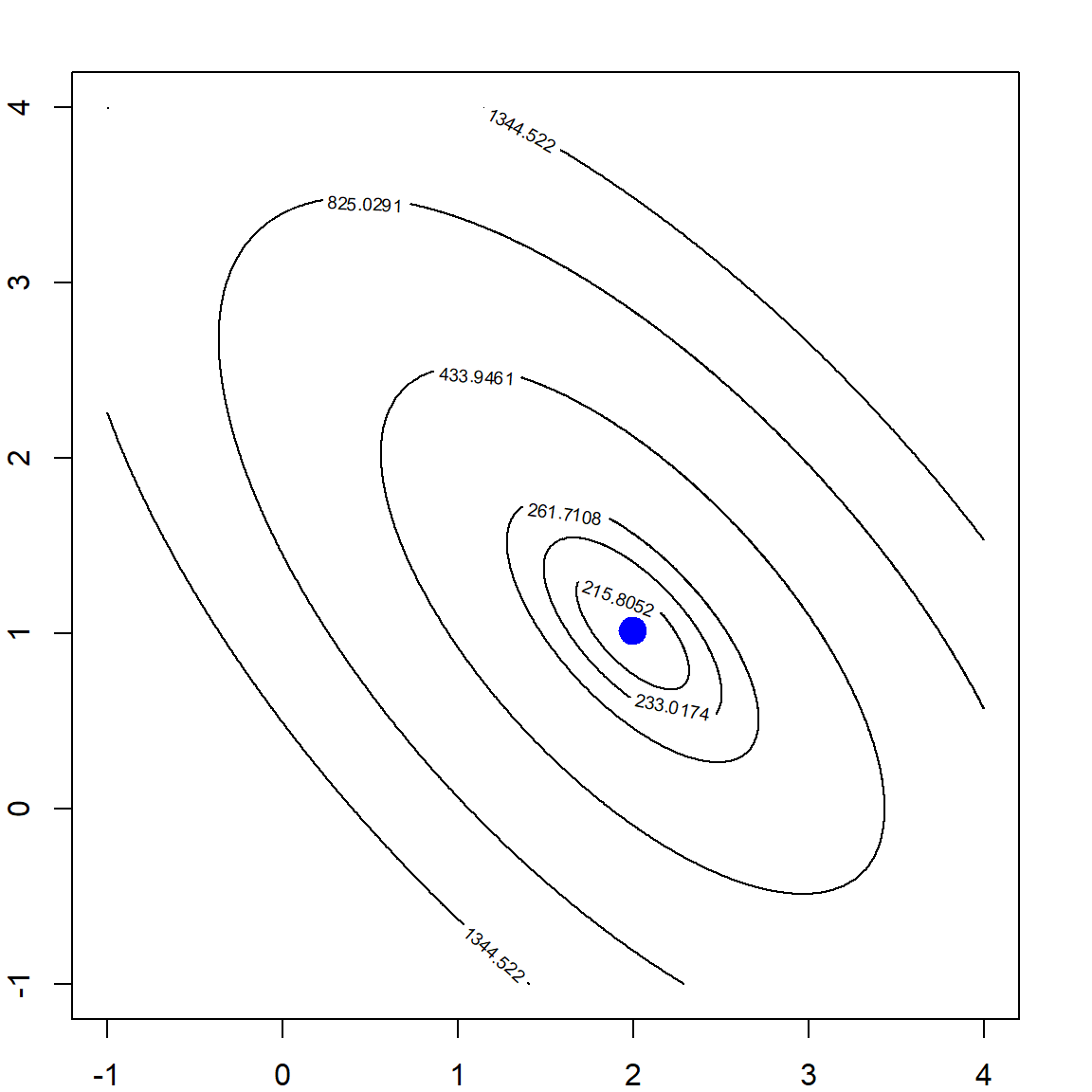
We use an optimization approach to solve this problem. By taking the derivative with respect to \(\boldsymbol \beta\), we have the gradient
\[ \begin{align} \frac{\partial \ell(\boldsymbol \beta)}{\partial \boldsymbol \beta} = -\frac{1}{n} \sum_{i=1}^n (y_i - x_i^\text{T} \boldsymbol \beta) x_i. \end{align} \] To perform the optimization, we will first set an initial beta value, say \(\boldsymbol \beta = \mathbf{0}\) for all entries, then proceed with the update
\[ \boldsymbol \beta^\text{new} = \boldsymbol \beta^\text{old} - \frac{\partial \ell(\boldsymbol \beta)}{\partial \boldsymbol \beta} \times \delta.\]
Let’s set \(\delta = 0.2\) for now. The following function performs gradient descent.
  # gradient descent function, which also record the path
  mylm_g <- function(x, y,
                     b0 = rep(0, ncol(x)), # initial value
                     delta = 0.2, # step size
                     epsilon = 1e-6, #stopping rule
                     maxitr = 5000) # maximum iterations
  {
    if (!is.matrix(x)) stop("x must be a matrix")
    if (!is.vector(y)) stop("y must be a vector")
    if (nrow(x) != length(y)) stop("number of observations different")

    # initialize beta values
    allb = matrix(b0, 1, length(b0))

    # iterative update
    for (k in 1:maxitr)
    {
      # the new beta value
      b1 = b0 + t(x) %*% (y - x %*% b0) * delta / length(y)

      # record the new beta
      allb = rbind(allb, as.vector(b1))

      # stopping rule
      if (max(abs(b0 - b1)) < epsilon)
        break;

      # reset beta0
      b0 = b1
    }

    if (k == maxitr) cat("maximum iteration reached\n")
    return(list("allb" = allb, "beta" = b1))
  }

  # fit the model
  mybeta = mylm_g(X, y, b0 = c(0, 1))

  par(bg="transparent")
  contour(beta1, beta2, rss, levels = quantile(rss, quanlvl))
  points(mybeta$allb[,1], mybeta$allb[,2], type = "b", col = "red", pch = 19)
  points(b[1], b[2], pch = 19, col = "blue", cex = 1.5)
  box()
The descent path is very smooth because we choose a very small step size. However, if the step size is too large, we may observe unstable results or even unable to converge. For example, if We set \(\delta = 1\) or \(\delta = 1.5\).
  par(mfrow=c(1,2))
  par(mar=c(2,2,2,2))

  # fit the model with a larger step size
  mybeta = mylm_g(X, y, b0 = c(0, 1), delta = 1)

  contour(beta1, beta2, rss, levels = quantile(rss, quanlvl))
  points(mybeta$allb[,1], mybeta$allb[,2], type = "b", col = "red", pch = 19)
  points(b[1], b[2], pch = 19, col = "blue", cex = 1.5)
  box()

  # and even larger
  mybeta = mylm_g(X, y, b0 = c(0, 1), delta = 1.5, maxitr = 6)
## maximum iteration reached

  contour(beta1, beta2, rss, levels = quantile(rss, quanlvl))
  points(mybeta$allb[,1], mybeta$allb[,2], type = "b", col = "red", pch = 19)
  points(b[1], b[2], pch = 19, col = "blue", cex = 1.5)
  box()
5.8 Coordinate Descent
Instead of updating all parameters at a time, we can also update one parameter each time. The Gauss-Seidel style coordinate descent algorithm at the \(k\)th iteration will sequentially update all \(p\) parameters:
\[\begin{align} x_1^{(k+1)} &= \underset{\color{OrangeRed}{x_1}}{\arg\min} \quad f(\color{OrangeRed}{x_1}, x_2^{(k)}, \ldots, x_p^{(k)}) \nonumber \\ x_2^{(k+1)} &= \underset{\color{OrangeRed}{x_2}}{\arg\min} \quad f(x_1^{\color{DodgerBlue}{(k+1)}}, \color{OrangeRed}{\mathbf{x}_2}, \ldots, x_p^{(k)}) \nonumber \\ \cdots &\nonumber \\ x_p^{(k+1)} &= \underset{\color{OrangeRed}{x_p}}{\arg\min} \quad f(x_1^{\color{DodgerBlue}{(k+1)}}, x_2^{\color{DodgerBlue}{(k+1)}}, \ldots, \color{OrangeRed}{x_p}) \nonumber \\ \end{align}\]
Note that after updating one coordinate, the new parameter value is used for updating the next coordinate. After we complete this loop, all \(j\) are updated to their new values, and we proceed to the next step.
Another type of update is the Jacobi style, which can be performed in parallel at the \(k\)th iteration:
\[\begin{align} x_1^{(k+1)} &= \underset{\color{OrangeRed}{x_1}}{\arg\min} \quad f(\color{OrangeRed}{x_1}, x_2^{(k)}, \ldots, x_p^{(k)}) \nonumber \\ x_2^{(k+1)} &= \underset{\color{OrangeRed}{x_2}}{\arg\min} \quad f(x_1^{(k+1)}, \color{OrangeRed}{\mathbf{x}_2}, \ldots, x_p^{(k)}) \nonumber \\ \cdots &\nonumber \\ x_p^{(k+1)} &= \underset{\color{OrangeRed}{x_p}}{\arg\min} \quad f(x_1^{(k+1)}, x_2^{(k+1)}, \ldots, \color{OrangeRed}{x_p}) \nonumber \\ \end{align}\]
For differentiable convex functions \(f\), we can ensure that if all parameters are optimized then the entire problem is also optimized. If \(f\) is not differentiable, we may have trouble (see the example on wiki). However, there are also cases where coordinate descent would still guarantee a convergence, e.g., a sperable case:
\[f(\mathbf{x}) = g(\mathbf{x}) + \sum_{j=1}^p h_j(x_j)\] This is the Lasso formulation which will be discussed in later section.
5.8.1 Coordinate Descent Example: Linear Regression
Coordinate descent for linear regression is not really necessary. However, we will still use this as an example. Note that the update for a single parameter is
\[ \underset{\boldsymbol \beta_j}{\text{argmin}} \frac{1}{2n} ||\mathbf{y}- X_j \beta_j - \mathbf{X}_{(-j)} \boldsymbol{\beta}_{(-j)} ||^2 \]
where \(\mathbf{X}_{(-j)}\) is the data matrix without the \(j\)th column. Note that when updating \(\beta_j\) coordinate-wise, we can first calculate the residual defined as \(\mathbf{r} = \mathbf{y} - \mathbf{X}_{(-j)} \boldsymbol \beta_{(-j)}\) which does not depend on \(\beta_j\), and optimize the rest of the formula for \(\beta_j\). This is essentially the same as performing a one-dimensional regression by regressing \(\mathbf{r}\) on \(X_j\) and obtain the update. \[ \beta_j = \frac{X_j^T \mathbf{r}}{X_j^T X_j} \] The coordinate descent usually does not involve choosing a step size. Note that the following function is NOT efficient because there are a lot of wasted calculations. It is only for demonstration purpose. Here we use the Gauss-Seidel style update.
  # gradient descent function, which also record the path
  mylm_c <- function(x, y, b0 = rep(0, ncol(x)), epsilon = 1e-6, maxitr = 5000)
  {
    if (!is.matrix(x)) stop("x must be a matrix")
    if (!is.vector(y)) stop("y must be a vector")
    if (nrow(x) != length(y)) stop("number of observations different")

    # initialize beta values
    allb = matrix(b0, 1, length(b0))

    # iterative update
    for (k in 1:maxitr)
    {
      # initiate a vector for new beta
      b1 = b0

      for (j in 1:ncol(x))
      {
        # calculate the residual
        r = y - x[, -j, drop = FALSE] %*% b1[-j]

        # update jth coordinate
        b1[j] = t(r) %*% x[,j] / (t(x[,j, drop = FALSE]) %*% x[,j])

        # record the update
        allb = rbind(allb, as.vector(b1))
      }

      if (max(abs(b0 - b1)) < epsilon)
        break;

      # reset beta0
      b0 = b1
    }

    if (k == maxitr) cat("maximum iteration reached\n")
    return(list("allb" = allb, "beta" = b1))
  }

  # fit the model
  mybeta = mylm_c(X, y, b0 = c(0, 3))

  par(mfrow=c(1,1))
  contour(beta1, beta2, rss, levels = quantile(rss, quanlvl))
  points(mybeta$allb[,1], mybeta$allb[,2], type = "b", col = "red", pch = 19)
  points(b[1], b[2], pch = 19, col = "blue", cex = 1.5)
  box()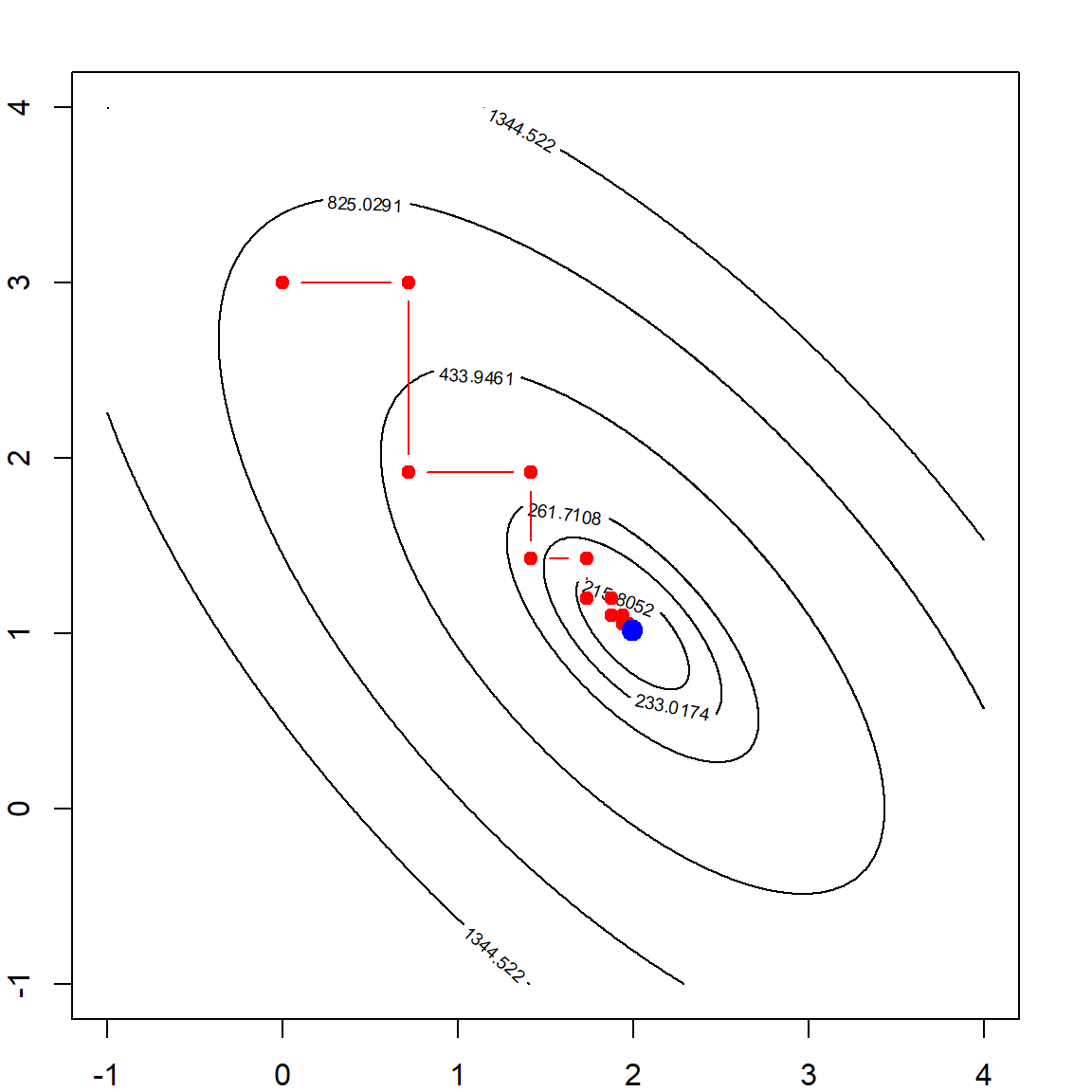
5.9 Stocastic Gradient Descent
The main advantage of using Stochastic Gradient Descent (SGD) is its computational speed. Calculating the gradient using all observations can be costly. Instead, we consider update the parameter based on a single observation. Hence, the gradient is defined as
\[ \frac{\partial \ell_i(\boldsymbol \beta)}{\partial \boldsymbol \beta} = - (y_i - x_i^\text{T} \boldsymbol \beta) x_i. \] Compared with using all observations, this is \(1/n\) of the cost. However, because this is rater not accurate for each iteration, but can still converge in the long run. There is a decay rate involved in SGD step size. If the step size does not decreases to 0, the algorithm cannot converge. However, it also has to sum up to infinite to allow us to go as far as we can. For example, a choice could be \(\delta_k = 1/k\), hence \(\sum \delta_k = \infty\) and \(\sum \delta_k^2 < \infty\).
  # gradient descent function, which also record the path
  mylm_sgd <- function(x, y, b0 = rep(0, ncol(x)), delta = 0.05, maxitr = 10)
  {
    if (!is.matrix(x)) stop("x must be a matrix")
    if (!is.vector(y)) stop("y must be a vector")
    if (nrow(x) != length(y)) stop("number of observations different")

    # initialize beta values
    allb = matrix(b0, 1, length(b0))

    # iterative update
    for (k in 1:maxitr)
    {
      # going through all samples
      for (i in sample(1:nrow(x)))
      {
        # update based on the gradient of a single subject
        b0 = b0 + (y[i] - sum(x[i, ] * b0)) * x[i, ] * delta

        # record the update
        allb = rbind(allb, as.vector(b0))

        # learning rate decay
        delta = delta * 1/k
      }
    }

    return(list("allb" = allb, "beta" = b0))
  }

  # fit the model
  mybeta = mylm_sgd(X, y, b0 = c(0, 1), maxitr = 3)

  contour(beta1, beta2, rss, levels = quantile(rss, quanlvl))
  points(mybeta$allb[,1], mybeta$allb[,2], type = "b", col = "red", pch = 19)
  points(b[1], b[2], pch = 19, col = "blue", cex = 1.5)
  box()
5.9.1 Mini-batch Stocastic Gradient Descent
Instead of using just one observation, we could also consider splitting the data into several small “batches” and use one batch of sample to calculate the gradient at each iteration.
  # gradient descent function, which also record the path
  mylm_sgd_mb <- function(x, y, b0 = rep(0, ncol(x)), delta = 0.3, maxitr = 20)
  {
    if (!is.matrix(x)) stop("x must be a matrix")
    if (!is.vector(y)) stop("y must be a vector")
    if (nrow(x) != length(y)) stop("number of observations different")

    # initiate batches with 10 observations each
    batch = sample(rep(1:floor(nrow(x)/10), length.out = nrow(x)))

    # initialize beta values
    allb = matrix(b0, 1, length(b0))

    # iterative update
    for (k in 1:maxitr)
    {
      for (i in 1:max(batch)) # loop through batches
      {
        # update based on the gradient of a single subject
        b0 = b0 + t(x[batch==i, ]) %*% (y[batch==i] - x[batch==i, ] %*% b0) *
          delta / sum(batch==i)

        # record the update
        allb = rbind(allb, as.vector(b0))

        # learning rate decay
        delta = delta * 1/k
      }
    }

    return(list("allb" = allb, "beta" = b0))
  }

  # fit the model
  mybeta = mylm_sgd_mb(X, y, b0 = c(0, 1), maxitr = 3)

  contour(beta1, beta2, rss, levels = quantile(rss, quanlvl))
  points(mybeta$allb[,1], mybeta$allb[,2], type = "b", col = "red", pch = 19)
  points(b[1], b[2], pch = 19, col = "blue", cex = 1.5)
  box()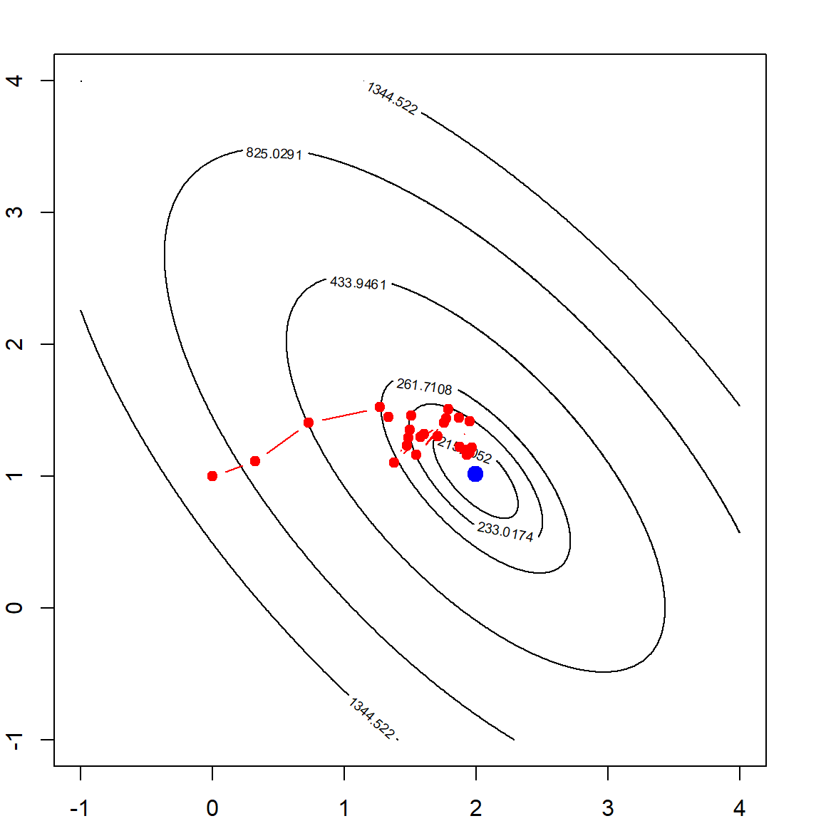
You may further play around with these tuning parameters to see how sensitive the optimization is to them. A stopping rule can be difficult to determine, hence in practice, early stop is also used.
5.10 Lagrangian Multiplier for Constrained Problems
Constrained optimization problems appear very frequently. Both Lasso and Ridge regressions can be viewed as constrained problems, while support vector machines (SVM) is another example, which will be introduced later on. Let’s investigate this using a toy example. Suppose we have an optimization problem
\[\text{minimize} \quad f(x, y) = x^2 + y^2\] \[\text{subj. to} \quad g(x, y) = xy - 4 = 0\]
  x <- seq(-5, 5, 0.05)
  y <- seq(-5, 5, 0.05)
  mygrid <- data.matrix(expand.grid(x, y))
  f <- matrix(mygrid[,1]^2 + mygrid[,2]^2, length(x), length(y))

  f2 <- matrix(mygrid[,1]*mygrid[,2], length(x), length(y))

  # plot the contour
  par(mar=c(2,2,2,2))
  contour(x, y, f, levels = c(0.2, 1, 2, 4, 8, 16))
  contour(x, y, f2, levels = 4, add = TRUE, col = "blue", lwd = 2)
  box()

  lines(seq(1, 3, 0.01), 4- seq(1, 3, 0.01), type = "l", col = "darkorange", lwd = 3)
  points(2, 2, col = "red", pch = 19, cex = 2)
  points(-2, -2, col = "red", pch = 19, cex = 2)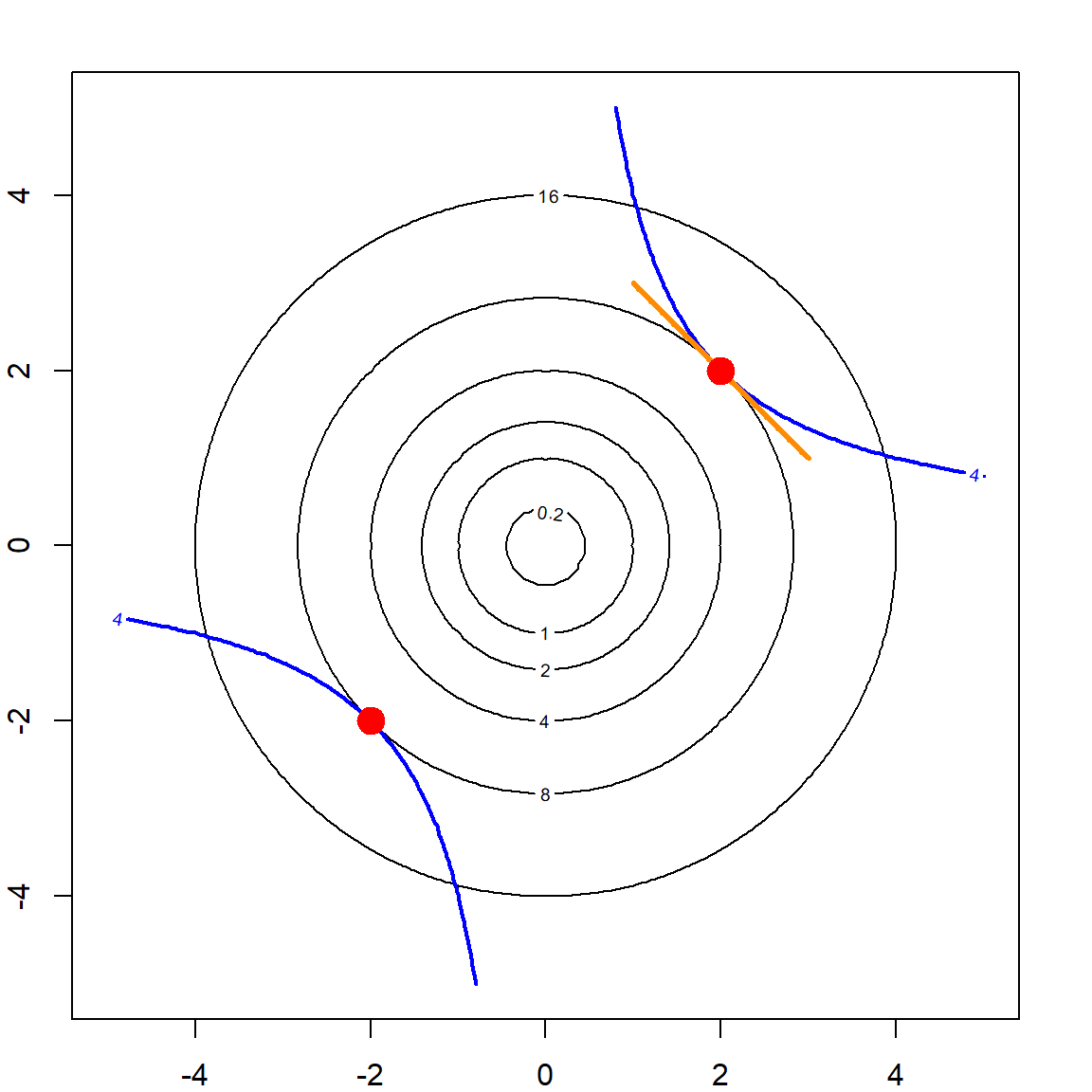
The problem itself is very simple. We know that the optimizer is the red dot. But an interesting point of view is to look at the level curves of the objective function. As it is growing (expanding), there is one point (the red dot) at which level curve barely touches the constrain curve (blue line). This should be the optimizer. But this also implies that the tangent line (orange line) of this leveling curve must coincide with the tangent line of the constraint. Noticing that the tangent line can be obtained by taking the derivative of the function, this observation implies that gradients of the two functions (the objective function and the constraint function) must be a multiple of the other. Hence,
\[ \begin{align} & \bigtriangledown f = \lambda \bigtriangledown g \\ \\ \Longrightarrow \qquad & \begin{cases} 2x = \lambda y & \text{by taking derivative w.r.t.} \,\, x\\ 2y = \lambda x & \text{by taking derivative w.r.t.} \,\, y\\ xy - 4 = 0 & \text{the constraint itself} \end{cases} \end{align} \]
The three equations put together is very easy to solve. We have \(x = y = 0\) or \(\lambda = \pm 2\) based on the first two equations. The first one is not feasible based on the constraint. The second solution leads to two feasible solutions: \(x = y = 2\) or \(x = y = -2\). Hence, we now know that there are two solutions.
Now, looking back at the equation \(\bigtriangledown f = \lambda \bigtriangledown g\), this is simply the derivative of the Lagrangian function defined as
\[{\cal L}(x, y, \lambda) = f(x, y) - \lambda g(x, y),\] while solving for the solution of the constrained problem becomes finding the stationary point of the Lagrangian. Be aware that in some cases, the solution you found can be maximizers instead of minimizers. Hence, its necessary to compare all of them and see which one is smaller.