Chapter 13 Kernel Smoothing
Fundamental ideas of local regression approaches are similar to \(k\)NN. But most approaches would address a fundamental drawback of \(k\)NN that the estimated function is not smooth. Having a smoothed estimation would also allow us to estimate the derivative, which is essentially used when estimating the density function. We will start with the intuition of the kernel estimator and then discuss the bias-variance trade-off using kernel density estimation as an example.
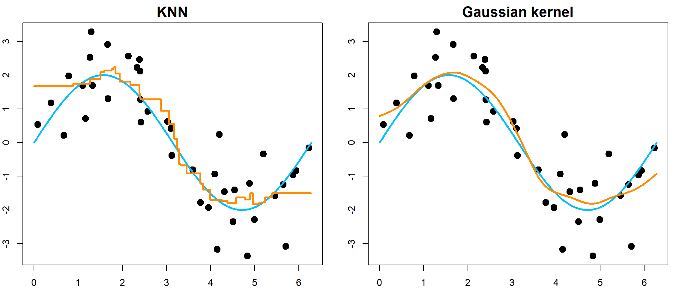
13.1 KNN vs. Kernel
We first compare the \(K\)NN method with a Gaussian kernel regression. \(K\)NN has jumps while Gaussian kernel regression is smooth.
13.2 Kernel Density Estimations
A natural estimator, by using the counts, is
\[\widehat f(x) = \frac{\#\big\{x_i: x_i \in [x - \frac{h}{2}, x + \frac{h}{2}]\big\}}{h n}\] This maybe compared with the histogram estimator
    library(ggplot2)
    data(mpg)

    # histogram
    hist(mpg$hwy, breaks = seq(6, 50, 2))

    # uniform kernel
    xgrid = seq(6, 50, 0.1)
    histden = sapply(xgrid, FUN = function(x, obs, h) sum( ((x-h/2) <= obs) * ((x+h/2) > obs))/h/length(obs),
                     obs = mpg$hwy, h = 2)

    plot(xgrid, histden, type = "s")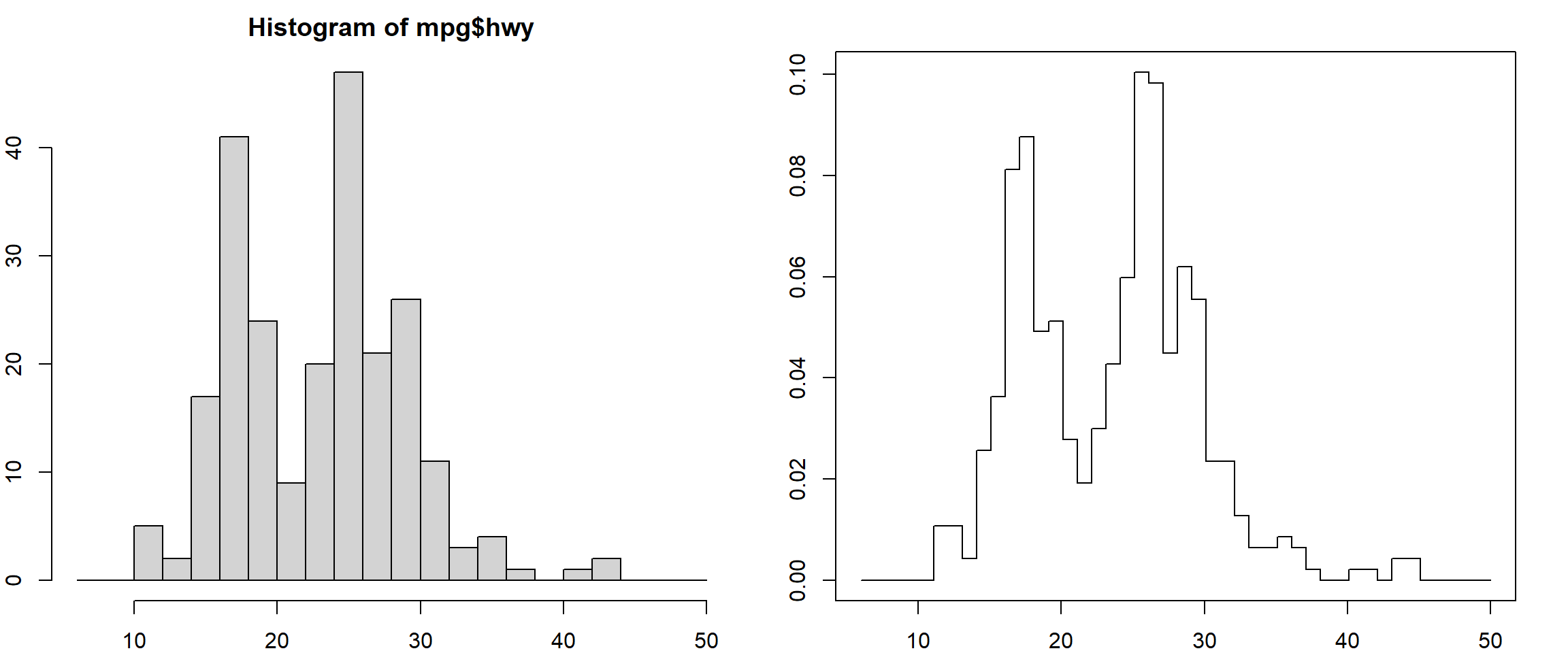
This can be view in two ways. The easier interpretation is that, for each target point, we count how many observations are close-by. We can also interpret it as evenly distributing the point-mass of each observation to a close-by region with width \(h\), and then stack them all.
\[\widehat f(x) = \frac{1}{h n} \sum_i \,\underbrace{ \mathbf{1} \Big(x \in [x_i - \frac{h}{2}, x_i + \frac{h}{2}]}_{\text{uniform density centered at } x_i} \Big)\] Here is a close-up demonstration of how those uniform density functions are stacked for all observations.
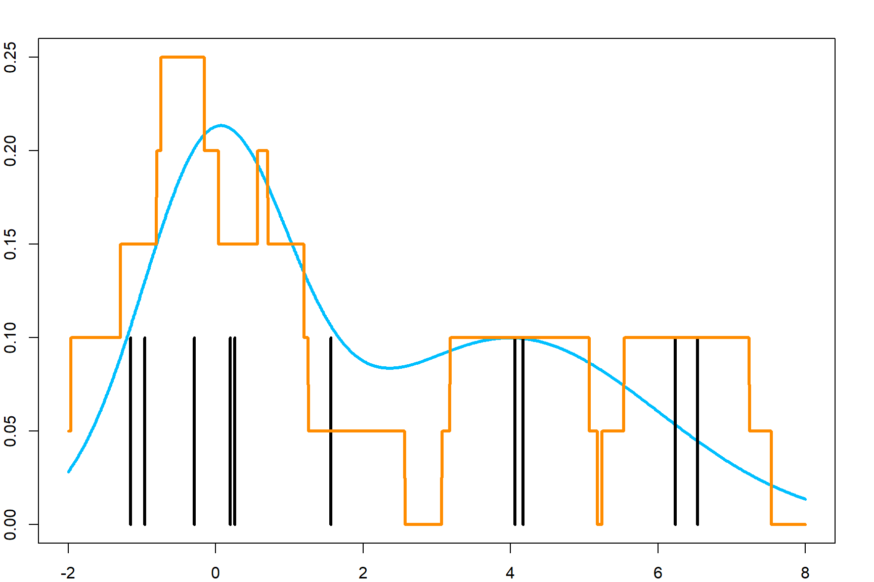
However, this is will lead to jumps at the end of each small uniform density. Let’s consider using a smooth function instead. Naturally, we can use the Gaussian kernel function to calculate the numerator in the above equation.
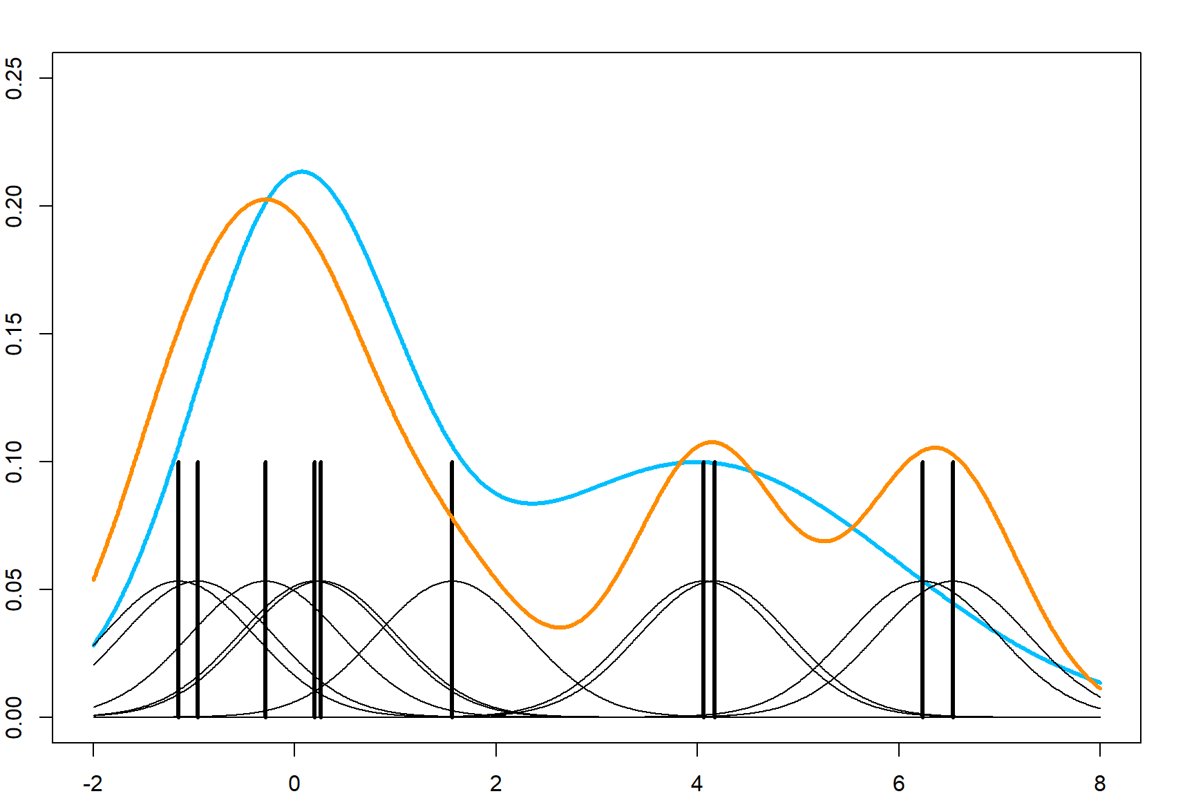
We apply this to the mpg dataset.
  xgrid = seq(6, 50, 0.1)
  kernelfun <- function(x, obs, h) sum(exp(-0.5*((x-obs)/h)^2)/sqrt(2*pi)/h)
  plot(xgrid, sapply(xgrid, FUN = kernelfun, obs = mpg$hwy, h = 1.5)/length(mpg$hwy), type = "l",
       xlab = "MPG", ylab = "Estimated Density", col = "darkorange", lwd = 3)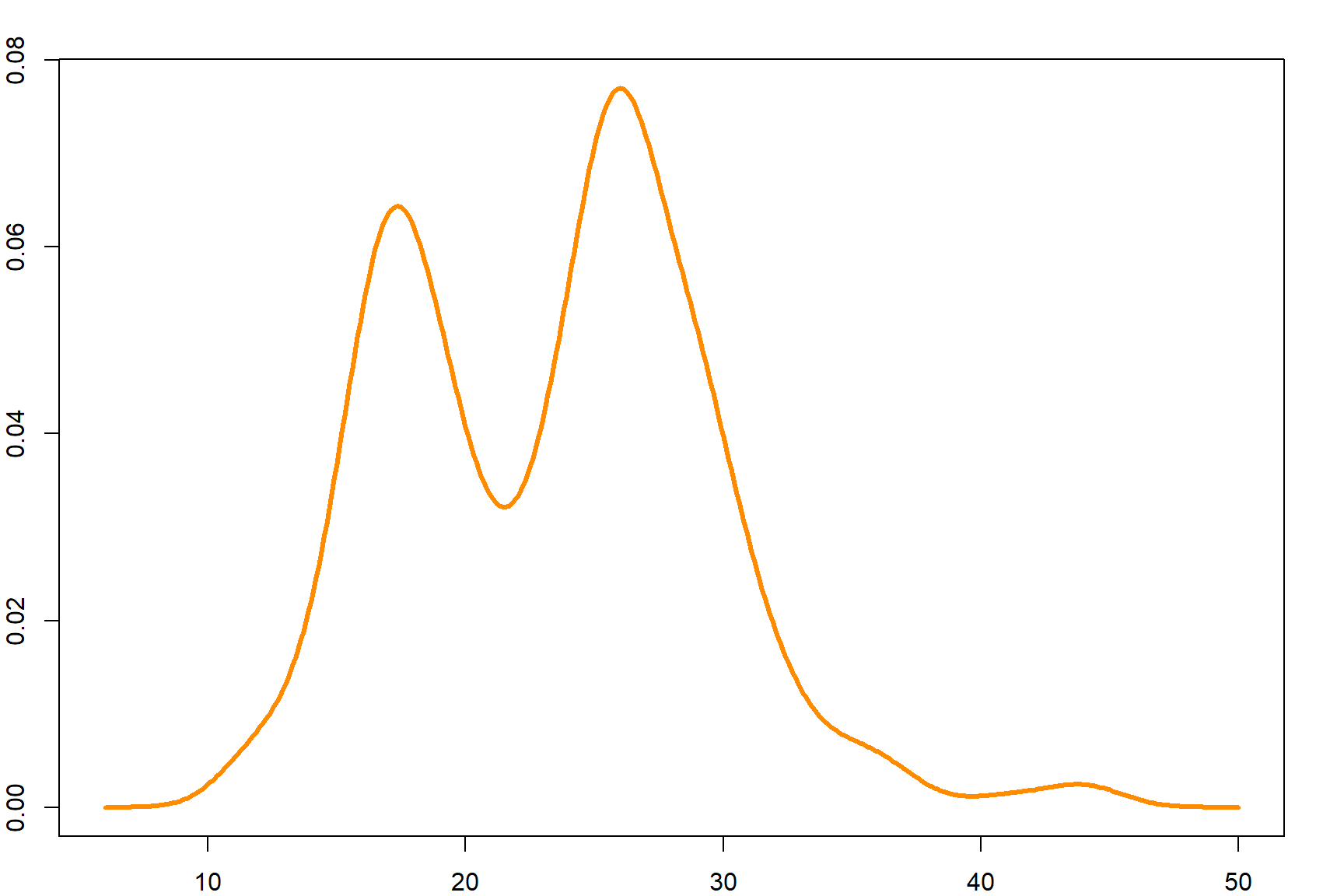
The ggplot2 packages provides some convenient features to plot the density and histogram.
  ggplot(mpg, aes(x=hwy)) +
    geom_histogram(aes(y=..density..), colour="black", fill="white")+
    geom_density(alpha=.2, fill="#ff8c00")
## Warning: The dot-dot notation (`..density..`) was deprecated in
## ggplot2 3.4.0.
## ℹ Please use `after_stat(density)` instead.
## This warning is displayed once every 8 hours.
## Call `lifecycle::last_lifecycle_warnings()` to see where
## this warning was generated.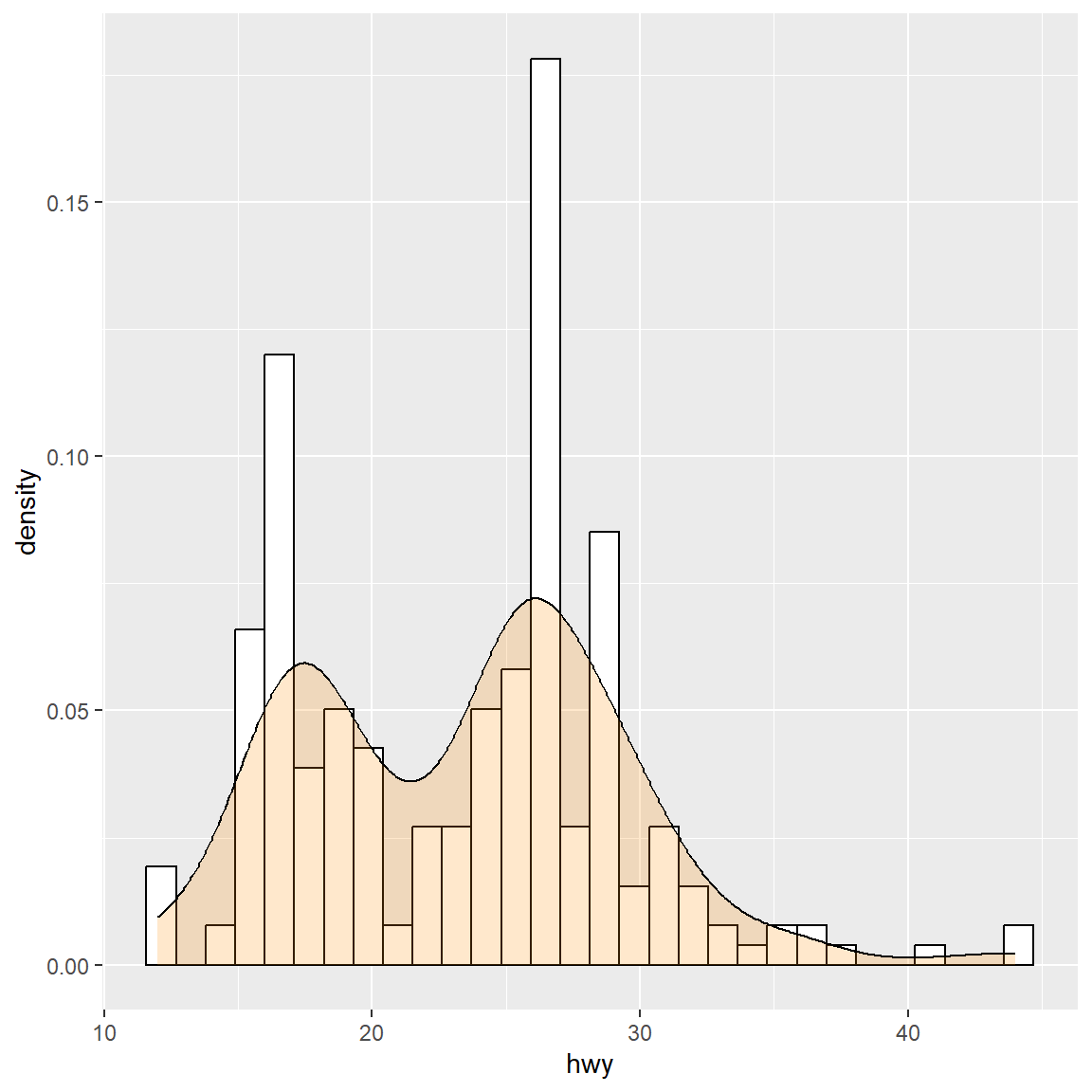
13.3 Expectation of the Parzen estimator
Let’s consider estimating a density, using the Parzen estimator
\[\widehat f(x) = \frac{1}{n} \sum_{i=1}^n K_{h} (x, x_i)\] The samples \(x_i\)’s are collected i.i.d. from a distribution with density \(f(x)\). Here, \(K_h(\mathbf{u}, \mathbf{v}) = K(|\mathbf{u}- \mathbf{v}|/h)/h\) is a kernel function, in which \(h\) scales the distance between \(x\) and \(x_i\) and adjust the smoothness of the density estimation accordingly. Our goal is to understand whether this estimator would converge to \(f(x)\) with reasonable conditions, provided that \(K(\cdot)\) is a proper density \(\int K(t) dt = 1\). First, we can analyze the bias:
\[\begin{align} \text{E}\big[ \widehat f(x) \big] &= \text{E}\left[ K\left( \frac{x - x_1}{h} \right) \Big/ h \right] \\ &= \int_{-\infty}^\infty \frac{1}{h} K\left(\frac{x-x_1}{h}\right) f(x_1) d x_1 \\ &= \int_{\infty}^{-\infty} \frac{1}{h} K(t) f(x - th) d (x-th) \\ &= \int_{-\infty}^\infty K(t) f(x - th) dt \\ (\text{as } h \rightarrow 0) \quad &\rightarrow f(x) \end{align}\]
In Chapter 14, we will provide a rigorous analysis the bias and variance, and show how an optimal bandwidth can be selected.
13.4 Gaussian Kernel Regression
A Nadaraya-Watson kernel regression model has the following formula. Note that we use \(h\) as the bandwidth instead of \(h\).
\[\widehat f(x) = \frac{\sum_i K_h(x, x_i) y_i}{\sum_i K_h(x, x_i)},\] where \(h\) is the bandwidth. At each target point \(x\), training data \(x_i\)s that are closer to \(x\) receives higher weights \(K_h(x, x_i)\), hence their \(y_i\) values are more influential in terms of estimating \(f(x)\). For the Gaussian kernel, we use
\[K_h(x, x_i) = \frac{1}{h\sqrt{2\pi}} \exp\left\{ -\frac{(x - x_i)^2}{2 h^2}\right\}\]
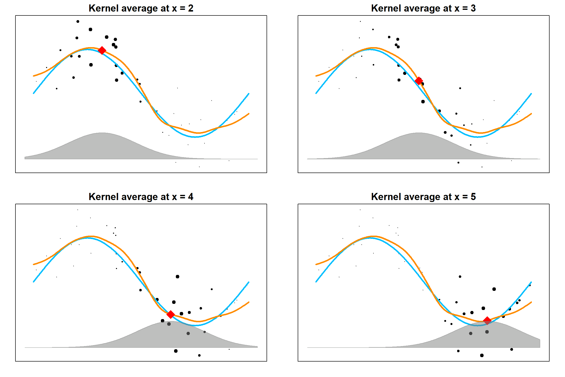
13.4.1 Bias-variance Trade-off
The bandwidth \(h\) is an important tuning parameter that controls the bias-variance trade-off. It behaves the same as the density estimation. By setting a large \(h\), the estimator is more stable but has more bias.
  # a small bandwidth
  ksmooth.fit1 = ksmooth(x, y, bandwidth = 0.5, kernel = "normal", x.points = testx)

  # a large bandwidth
  ksmooth.fit2 = ksmooth(x, y, bandwidth = 2, kernel = "normal", x.points = testx)

  # plot both
  plot(x, y, xlim = c(0, 2*pi), pch = 19, xaxt='n', yaxt='n')
  lines(testx, 2*sin(testx), col = "deepskyblue", lwd = 3)
  lines(testx, ksmooth.fit1$y, type = "s", col = "darkorange", lwd = 3)
  lines(testx, ksmooth.fit2$y, type = "s", col = "red", lwd = 3)
  legend("topright", c("h = 0.5", "h = 2"), col = c("darkorange", "red"),
         lty = 1, lwd = 2, cex = 1.5)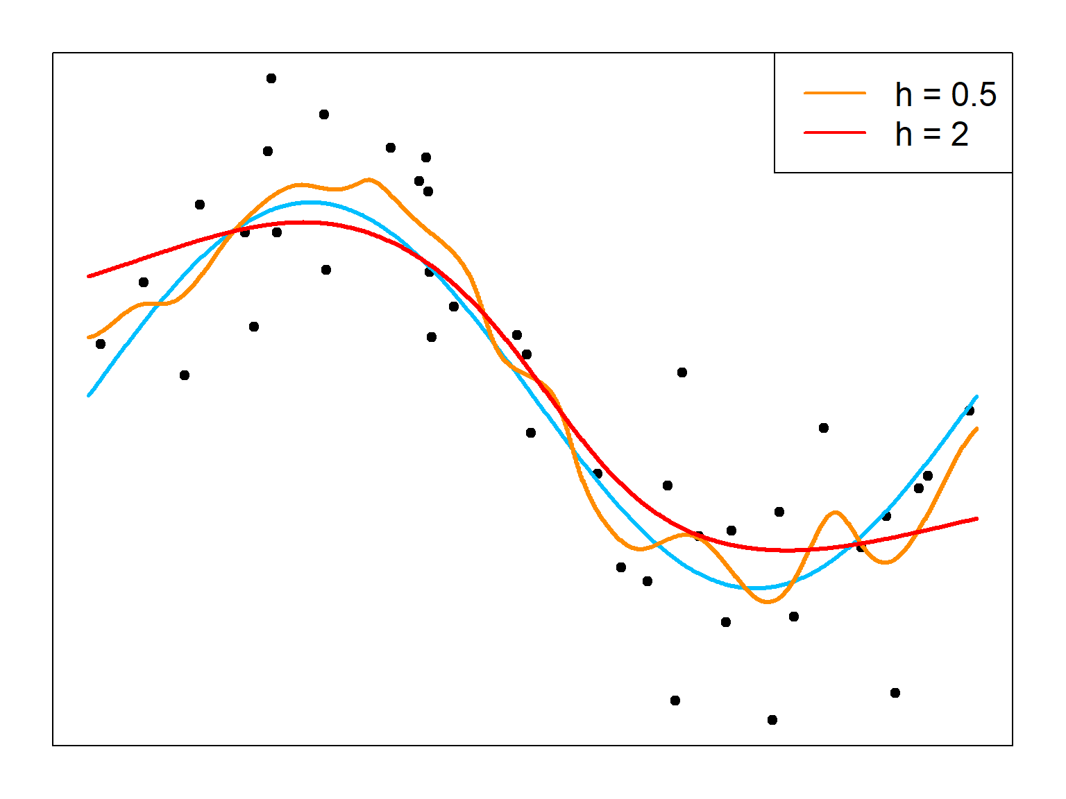
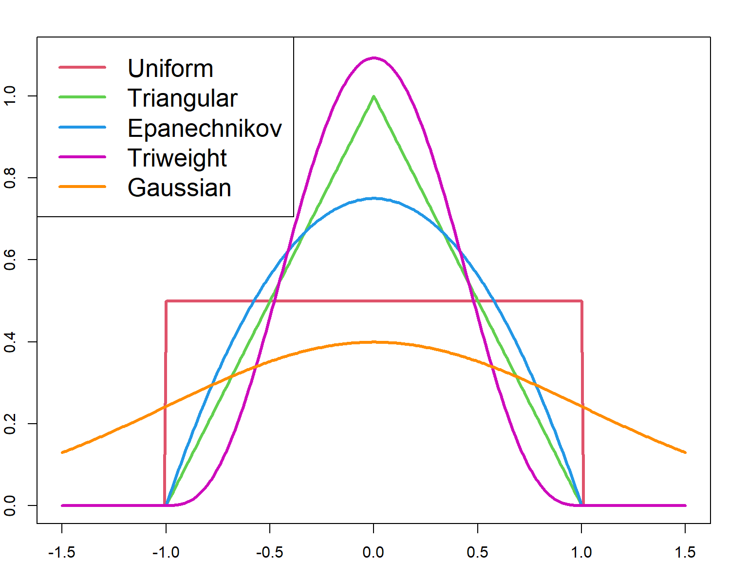
13.5 Choice of Kernel Functions
Other kernel functions can also be used. The most efficient kernel is the Epanechnikov kernel, which will minimize the mean integrated squared error (MISE). The efficiency is defined as
\[ \Big(\int u^2K(u) du\Big)^\frac{1}{2} \int K^2(u) du, \] Different kernel functions can be visualized in the following. Most kernels are bounded within \([-h/2, h/2]\), except the Gaussian kernel.
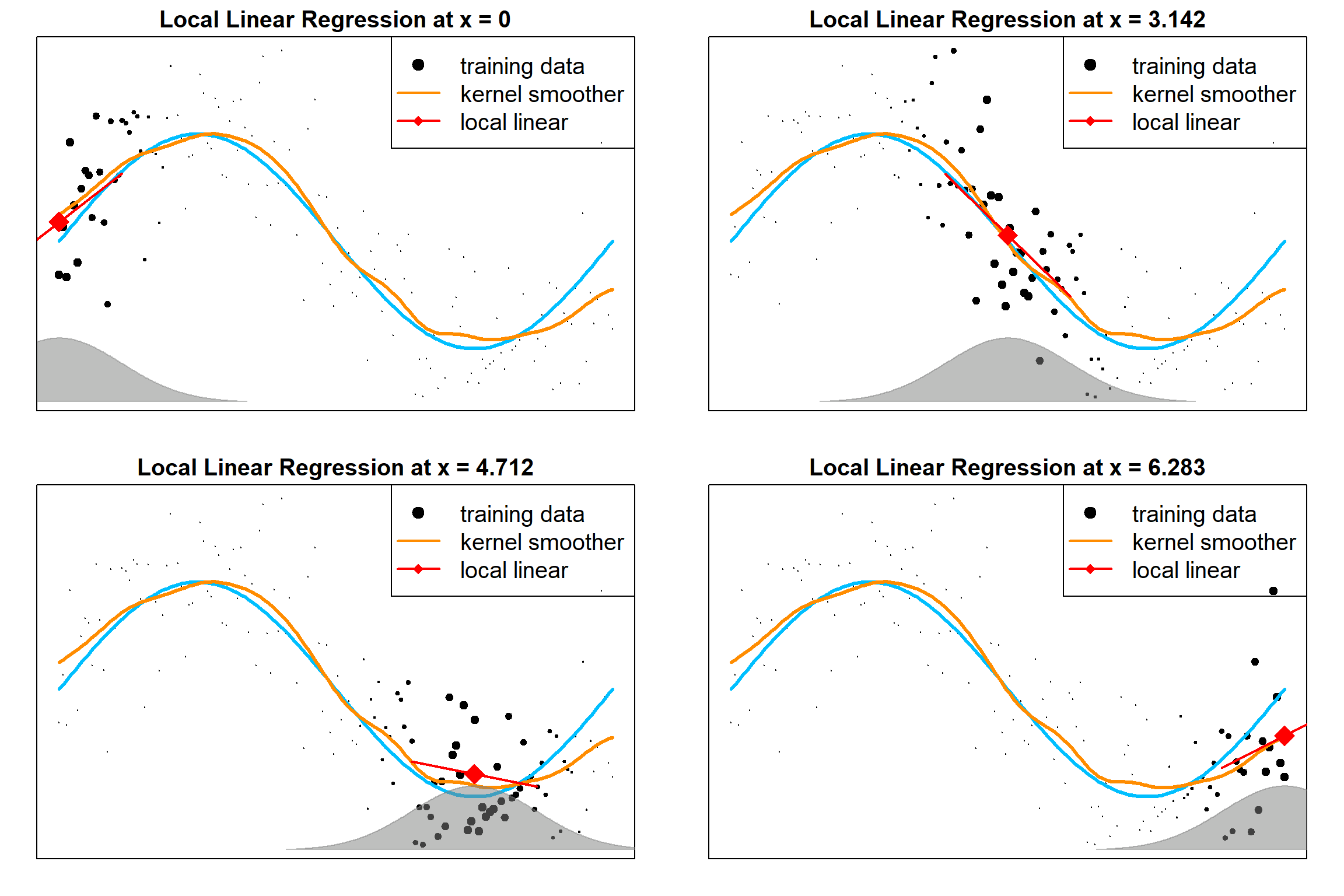
13.6 Local Linear Regression
Local averaging will suffer severe bias at the boundaries. One solution is to use the local polynomial regression. The following examples are local linear regressions, evaluated as different target points. We are solving for a linear model weighted by the kernel weights
\[\sum_{i = 1}^n K_h(x, x_i) \big( y_i - \beta_0 - \beta_1 x_i \big)^2\]
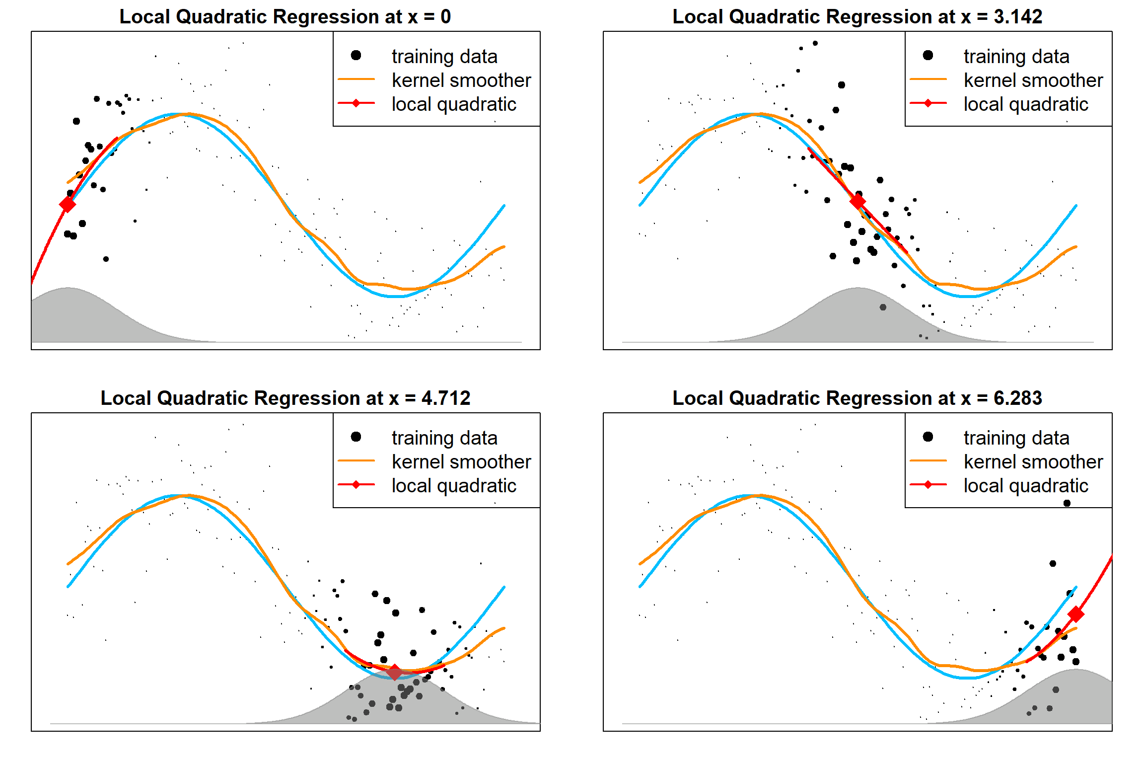
13.7 Local Polynomial Regression
The following examples are local polynomial regressions, evaluated as different target points. We can easily extend the local linear model to inccorperate higher orders terms:
\[\sum_{i=1}^n K_h(x, x_i) \Big[ y_i - \beta_0(x) - \sum_{r=1}^d \beta_j(x) x_i^r \Big]^2\]
The followings are local quadratic fittings, which will further correct the bias.
13.8 R Implementations
Some popular R functions implements the local polynomial regressions: loess, locfit, locploy, etc. These functions automatically calculate the fitted value for each target point (essentially all the observed points). This can be used in combination with ggplot2. The point-wise confidence intervals are also calculated.
    ggplot(mpg, aes(displ, hwy)) + geom_point() +
      geom_smooth(col = "red", method = "loess", span = 0.5)
## `geom_smooth()` using formula = 'y ~ x'
A toy example that compares different bandwidth. Be careful that different methods may formulat the bandwidth parameter in different ways.
    # local polynomial fitting using locfit and locpoly

    library(KernSmooth)
    library(locfit)

    n <- 100
    x <- runif(n,0,1)
    y <- sin(2*pi*x)+rnorm(n,0,1)
    y = y[order(x)]
    x = sort(x)

    plot(x, y, pch = 19)
    points(x, sin(2*pi*x), lwd = 3, type = "l", col = 1)
    lines(locpoly(x, y, bandwidth=0.15, degree=2), col=2, lwd = 3)
    lines(locfit(y~lp(x, nn = 0.3, h=0.05, deg=2)), col=4, lwd = 3)

    legend("topright", c("locpoly", "locfit"), col = c(2,4), lty = 1, cex = 1.5, lwd =2)