Chapter 18 The Representer Theorem
Previously, we have established several important properties of RKHS
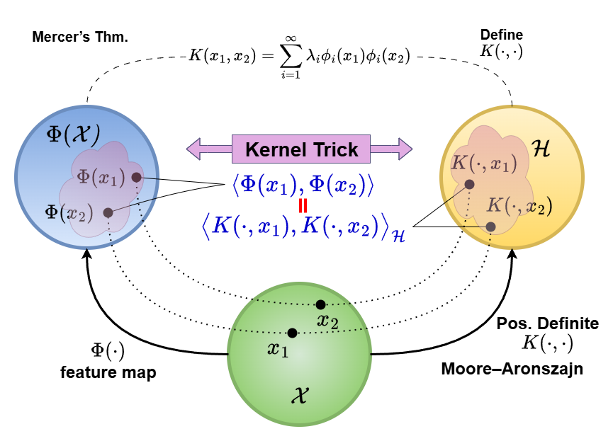
- The Moore–Aronszajn theorem (Aronszajn 1950) established the one-to-one correspondence between positive definite kernels and RKHS. We also know how to construct the RKHS given a kernel function.
- The Kernel trick (in SVM) allows us to compute inner products in an RKHS without explicitly mapping data points to the high-dimensional feature space.
- The Mercer theorem (Mercer 1909) provided a way to characterize a kernel with eigenfunctions and eigenvalues, giving another concrete example of such feature mappings with any positive definite kernel.
The connections of them can be illustrated using the following figure:
With these understandings, we want to further discuss how to computationally leverage the RKHS structure in statistical learning problems. Essentially, this is the goal of the Representer Theorem (Kimeldorf and Wahba 1970), which states that the solution to a large class of optimization problems in an RKHS can be represented as a finite linear combination of kernel functions evaluated at the training data points. Note that our previous spline example is a special case of this theorem. This is a powerful result because it allows us to reduce infinite-dimensional optimization problems to finite-dimensional ones, making them computationally feasible.
18.1 The Representer Theorem
\(\cal H\) is a very large space of functions. It is not clear if we want to find \(f\) in \(\cal H\) for our optimization problem, how do we computationally complete that task (think about the second-order Sobolev space example in smoothing spline). It is impossible to exhaust all such functions. Luckily, we don’t need to. This is ensured by the Representer Theorem, which states that only a finite sample presentation is needed.
The Representer Theorem If we are given a set of data \(\{x_i, y_i\}_{i=1}^n\), and we search for the best solution in \({\cal H}\) of the optimization problem \[ \widehat f = \underset{f \in \cal H}{\arg\min} \,\, {\cal L}(\{y_i, f(x_i)\}_{i=1}^n) + p(\| f \|_{{\cal H}}^2 ), \] where \({\cal L}\) is the loss function, \(p\) is a monotone penalty function, and \({\cal H}\) is the RKHS with kernel \(K\). Then the solution must take the form \[ \widehat f = \sum_{i=1}^n \alpha_i K(\cdot, x_i) \]
The proof is quite simple. The logic is the same as the smoothing spline proof. We can first use the kernel \(K\) associated with \(\cal H\) to define a set of functions \[K(\cdot, x_i), \, K(\cdot, x_2), \, \cdots, \, K(\cdot, x_n)\]
Remember that these functions defined on the observed data would define a finite-dimensional subspace \(\cal S\) of \(\cal H\). Then, suppose the (optimal) solution is some function \(f \in {\cal H}\), we can decompose it to the sum of functions in \(\cal S\) and its orthogonal complement \(\cal S^{\perp}\). In particular, we can write \(f\) as
\[f(\cdot) = \sum_{i=1}^n \alpha_i K(\cdot, x_i) + h(\cdot)\]
for some \(\alpha_i\) and \(h(\cdot)\). Here the orthogonal complement means the following. Let \({\cal S} = \text{span}\{K(\cdot, x_i), \, i=1, \cdots, n\}\) be the space spanned by these functions. Then the orthogonal complement of \(\cal S\) is defined as
\[ \cal S^{\perp} = \{ h \in \cal H : \langle h, g \rangle_{\cal H} = 0, \, \forall g \in \cal S \} \]
Such decomposition is always possible since \(\cal H\) is a Hilbert space5. Now we can investigate what happens to the loss function and the penalty term in the optimization problem. For the loss function, we only care about the values of \(f\) at the observed data points \(x_i\)’s. Note that the inner product between \(h(\cdot)\) and any function in \(\cal S\) has to be zero, we utilize the reproducing property to see that
\[ h(x_j) = \langle K(x_j, \cdot), h(\cdot) \rangle = 0 \]
for all \(j\). Or more explicitly, we have
\[\begin{align} f(x_j) =& \langle f(\cdot), K(\cdot, x_j) \rangle \nonumber \\ =& \left\langle \sum_{i=1}^n \alpha_i K(x_i, \cdot) + h(\cdot), K(\cdot, x_j) \right\rangle \nonumber \\ =& \sum_{i=1}^n \alpha_i K(x_i, x_j) + h(x_j) \nonumber \\ =& \sum_{i=1}^n \alpha_i K(x_i, x_j) \end{align}\]
This means that our finite sample representation already captures all the information of \(f\) at the observed data points. Hence, the loss function would be the same if we just use the finite sample representation without \(h(\cdot)\).
For the penalty term, we can see that
\[\begin{align} \lVert f \rVert^2_{\cal H}=& \lVert \sum_{i=1}^n \alpha_i K(\cdot, x_i) + h(\cdot) \rVert^2_{\cal H}\nonumber \\ =& \lVert \sum_{i=1}^n \alpha_i K(\cdot, x_i) \rVert^2_{\cal H}+ \lVert h(\cdot) \rVert^2_{\cal H} + 2 \sum_{i=1}^n \alpha_i \langle K(\cdot, x_i), h(\cdot) \rangle_{\cal H}\nonumber \\ =& \lVert \sum_{i=1}^n \alpha_i K(\cdot, x_i) \rVert^2_{\cal H}+ \lVert h(\cdot) \rVert^2_{\cal H} + 0 \nonumber \\ \geq& \lVert \sum_{i=1}^n \alpha_i K(\cdot, x_i) \rVert^2_{\cal H} \end{align}\]
This completes the proof since this finite represetnation would be the one being preferred than \(f\).
18.2 Notes on Application
The main computational implication of the Representer Theorem is that optimization problems in an RKHS can always be reduced to finite-dimensional problems involving the kernel matrix. In practice, this means that we only need to solve for the coefficients \(\boldsymbol{\alpha}= c(\alpha_1,\dots,\alpha_n)^\text{T}\) in the representation
\[ {\cal L}\Big(\{y_i, \sum_{j=1}^n \alpha_i K(x_i, x_j)\}_{i=1}^n \Big) + \lambda \boldsymbol{\alpha}^\text{T}\mathbf{K}\boldsymbol{\alpha}, \]
Here, we choose a very simple version of the penalty function as the Hilbert norm squared, i.e.,
\[ \|f\|_{\cal H}^2 = \langle f, f \rangle_{\cal H} = \sum_{i=1}^n \sum_{j=1}^n \alpha_i \alpha_j K(x_i, x_j) = \alpha^T K \alpha, \]
Typically, these parameters can be solved with standard optimization techniques. And furthermore, by penalizing the norm of the function in the RKHS, we are effectively controlling the complexity of the function. This is ensured by the smoothness properties of functions in an RKHS, provided in our previous notes.
Reference
To see a concrete (but maybe sloppy) example of this decomposition, recall the second-order Sobolev space in the smoothing spline example. If we consider any function \(f(\cdot)\), we may find a linear combination of \(\{K(\cdot, x_i)\}_{i=1}^n\) such that the difference between \(f\) and this linear combination has zero values at all \(x_i\)’s. But be careful that this does not necessarily mean that the kernel matrix needs to be full rank (Gaussian kernel is, but polynomial kernel may not be). The linear kernel will have rank \(p\), but the true function \(f\) can only live in the \(p\)-dimensional linear space. Hence, the linear combination of the kernel functions is still sufficient to represent \(f\) at those points. Now, this means that the difference between the two is \[ h(\cdot) = f(\cdot) - \sum_{i=1}^n \alpha_i K(\cdot, x_i) \] and \(h(x_i) = 0\) for all \(i\). Then, by the reproducing property, we have that \(h(\cdot)\) can be expressed as inner product, which has be zero: \[ 0 = h(x_i) = \langle K(x_i, \cdot), h(\cdot) \rangle \] for all \(i\). This means that \(h(\cdot)\) must be living in the orthogonal complement of the space spanned by \(\{K(\cdot, x_i)\}_{i=1}^n\) by the definition. As an additional note, the kernel matrix of a linear kernel is \(K = X X^T\), which has rank \(\min(n, p)\).↩︎