RLT Package Testing Regression Functions and Features
Ruoqing Zhu
Last Updated: July 17, 2025
Test-Reg.RmdInstall and Load Package
Install and load the GitHub version of the RLT package. Do not use the CRAN version.
  # install.packages("devtools")
  # devtools::install_github("teazrq/RLT")
  library(RLT)
## RLT and Random Forests v4.2.6
## pre-release at github.com/teazrq/RLT
Load other packages used in this guide.
Benchmark Against Existing Packages
We generate a dataset with 1000 observations and 400 variables, with 200 continuous variables and 200 categorical ones with three categories.
  library(parallel)
  # Set seed for reproducibility
  set.seed(1)

  # Define data size
  trainn <- 800
  testn <- 1000
  n <- trainn + testn
  p <- 30

  # Generate continuous variables (X1) and categorical variables (X2)
  X1 <- matrix(rnorm(n * p / 2), n, p / 2)
  X2 <- matrix(as.integer(runif(n * p / 2) * 3), n, p / 2)

  # Combine continuous and categorical variables into a data frame (X)
  X <- data.frame(X1, X2)

  # Convert the second half of the columns in X to factors
  X[, (p / 2 + 1):p] <- lapply(X[, (p / 2 + 1):p], as.factor)

  # Generate outcomes (y)
  y <- 1 + rowSums(X[, 2:6]) + 2 * (X[, p / 2 + 1] %in% c(1, 3)) + rnorm(n)

  # Set tuning parameters
  ntrees <- 1000
  ncores <- detectCores() - 1
  nmin <- 30
  mtry <- p / 2
  samplereplace <- TRUE
  sampleprob <- 0.80
  rule <- "best"
  nsplit <- ifelse(rule == "best", 0, 3)
  importance <- TRUE

  # Split data into training and testing sets
  trainX <- X[1:trainn, ]
  trainY <- y[1:trainn]
  testX <- X[(trainn + 1):(trainn + testn), ]
  testY <- y[(trainn + 1):(trainn + testn)]
  # recording results
  metric = data.frame(matrix(NA, 4, 6))
  rownames(metric) = c("RLT", "randomForestSRC", "randomForest", "ranger")
  colnames(metric) = c("fit.time", "pred.time", "oob.error", "pred.error",
                       "obj.size", "tree.size")

  # using RLT package
  start_time <- Sys.time()
  RLTfit <- RLT(trainX, trainY, model = "regression",
                ntrees = ntrees, mtry = mtry, nmin = nmin,
                resample.prob = sampleprob, split.gen = rule,
                resample.replace = samplereplace,
                nsplit = nsplit, importance = importance,
                param.control = list("alpha" = 0),
                ncores = ncores, verbose = TRUE)
## Regression Random Forest ...
## ---------- Parameters Summary ----------
##               (N, P) = (800, 30)
##           # of trees = 1000
##         (mtry, nmin) = (15, 30)
##       split generate = Best
##             sampling = 0.8 w/ replace
##   (Obs, Var) weights = (No, No)
##           importance = permute
##        reinforcement = No
## ----------------------------------------
  metric[1, 1] = difftime(Sys.time(), start_time, units = "secs")
  start_time <- Sys.time()
  RLTPred <- predict(RLTfit, testX, ncores = ncores)
  metric[1, 2] = difftime(Sys.time(), start_time, units = "secs")
  metric[1, 3] = mean((RLTfit$Prediction - trainY)^2)
  metric[1, 4] = mean((RLTPred$Prediction - testY)^2)
  metric[1, 5] = object.size(RLTfit)
  metric[1, 6] = mean(unlist(lapply(RLTfit$FittedForest$SplitVar, length)))

  # use randomForestSRC
  options(rf.cores = ncores)
  start_time <- Sys.time()
  rsffit <- rfsrc(y ~ ., data = data.frame(trainX, "y"= trainY),
                  ntree = ntrees, nodesize = nmin/2, mtry = mtry,
                  samptype = ifelse(samplereplace == TRUE, "swor", "swr"),
                  nsplit = nsplit, sampsize = trainn*sampleprob,
                  importance = ifelse(importance, "permute", "none"))
  metric[2, 1] = difftime(Sys.time(), start_time, units = "secs")
  start_time <- Sys.time()
  rsfpred = predict(rsffit, data.frame(testX))
  metric[2, 2] = difftime(Sys.time(), start_time, units = "secs")
  metric[2, 3] = mean((rsffit$predicted.oob - trainY)^2)
  metric[2, 4] = mean((rsfpred$predicted - testY)^2)
  metric[2, 5] = object.size(rsffit)
  metric[2, 6] = rsffit$forest$totalNodeCount / rsffit$ntree

  # use randomForest
  start_time <- Sys.time()
  rf.fit <- randomForest(trainX, trainY, ntree = ntrees,
                         mtry = mtry, nodesize = nmin,
                         replace = samplereplace,
                         sampsize = trainn*sampleprob,
                         importance = importance)
  metric[3, 1] = difftime(Sys.time(), start_time, units = "secs")
  start_time <- Sys.time()
  rf.pred <- predict(rf.fit, testX)
  metric[3, 2] = difftime(Sys.time(), start_time, units = "secs")
  metric[3, 3] = mean((rf.fit$predicted - trainY)^2)
  metric[3, 4] = mean((rf.pred - testY)^2)
  metric[3, 5] = object.size(rf.fit)
  metric[3, 6] = mean(colSums(rf.fit$forest$nodestatus != 0))


  # use ranger
  start_time <- Sys.time()
  rangerfit <- ranger(trainY ~ ., data = data.frame(trainX),
                      num.trees = ntrees, min.node.size = nmin,
                      mtry = mtry, num.threads = ncores,
                      replace = samplereplace,
                      sample.fraction = sampleprob,
                      importance = "permutation",
                      respect.unordered.factors = "partition")
  metric[4, 1] = difftime(Sys.time(), start_time, units = "secs")
  start_time <- Sys.time()
  rangerpred = predict(rangerfit, data.frame(testX))
  metric[4, 2] = difftime(Sys.time(), start_time, units = "secs")
  metric[4, 3] = mean((rangerfit$predictions - trainY)^2)
  metric[4, 4] = mean((rangerpred$predictions - testY)^2)
  metric[4, 5] = object.size(rangerfit)
  metric[4, 6] = mean(unlist(lapply(rangerfit$forest$split.varIDs, length)))

  # performance summary
  metric
##                  fit.time  pred.time oob.error pred.error obj.size tree.size
## RLT             0.7899787 0.04829931  2.326833   2.348519  4855800    79.080
## randomForestSRC 2.3519471 0.15868258  2.329721   2.417986 13419416    81.296
## randomForest    3.5314641 0.05414748  2.327304   2.372427  3212440    79.312
## ranger          1.3993149 0.07059932  2.318683   2.358706  2842856    79.352
Print a Single Tree
You can use the get.one.tree() function to peek into a
single tree.
  get.one.tree(RLTfit, 1)
## Tree #1 in the fitted regression forest:
##     SplitVar SplitValue LeftNode RightNode NodeWeight     NodeAve
## 1        X2   0.5130879        2         3        640  0.00000000
## 2        X5   0.1245613        4         5        461  0.00000000
## 3        X4   0.1278372       68        69        179  0.00000000
## 4        X6  -0.9315267        6         7        270  0.00000000
## 5        X3  -0.3566060       36        37        191  0.00000000
## 6        X3  -0.6818253        8         9         52  0.00000000
## 7        X2  -1.1202194       12        13        218  0.00000000
## 8       <NA>         NA       NA        NA         20 -4.05831582
## 9       X13   0.6969620       10        11         32  0.00000000
## 10      <NA>         NA       NA        NA         25 -1.56610269
## 11      <NA>         NA       NA        NA          7  0.33467263
## 12      X11   0.8086734       14        15         49  0.00000000
## 13       X5  -1.9740546       18        19        169  0.00000000
## 14       X4  -1.2378102       16        17         32  0.00000000
## 15      <NA>         NA       NA        NA         17  0.83807065
## 16      <NA>         NA       NA        NA          4 -5.07730369
## 17      <NA>         NA       NA        NA         28 -1.16601538
## 18      <NA>         NA       NA        NA         15 -1.75654440
## 19  X1.1 (F)  4.0000000       20        21        154  0.00000000
## 20       X6   0.2068412       22        23         94  0.00000000
## 21       X5  -0.8397821       30        31         60  0.00000000
## 22       X3  -0.2591860       24        25         54  0.00000000
## 23       X7  -0.9688096       28        29         40  0.00000000
## 24      <NA>         NA       NA        NA         17 -1.33291805
## 25 X14.1 (F)  4.0000000       26        27         37  0.00000000
## 26      <NA>         NA       NA        NA         18 -0.43713880
## 27      <NA>         NA       NA        NA         19  0.94011843
## 28      <NA>         NA       NA        NA         17  2.53305108
## 29      <NA>         NA       NA        NA         23  0.66413456
## 30      <NA>         NA       NA        NA         22  0.85873903
## 31      X12  -1.8288810       32        33         38  0.00000000
## 32      <NA>         NA       NA        NA          3  4.32370542
## 33      X13   0.7978382       34        35         35  0.00000000
## 34      <NA>         NA       NA        NA         26  2.58142104
## 35      <NA>         NA       NA        NA          9  1.49224825
## 36       X3  -2.0974592       38        39         70  0.00000000
## 37       X4  -0.1241238       52        53        121  0.00000000
## 38      <NA>         NA       NA        NA          4 -2.32649240
## 39       X6  -0.7842442       40        41         66  0.00000000
## 40      <NA>         NA       NA        NA          9 -1.03000167
## 41       X6  -0.7207343       42        43         57  0.00000000
## 42      <NA>         NA       NA        NA          3  4.06230418
## 43      X12  -0.3962172       44        45         54  0.00000000
## 44      <NA>         NA       NA        NA         13  2.51658857
## 45       X3  -0.4572172       46        47         41  0.00000000
## 46       X4   0.4462492       48        49         39  0.00000000
## 47      <NA>         NA       NA        NA          2  3.21089666
## 48      X13  -0.9595361       50        51         32  0.00000000
## 49      <NA>         NA       NA        NA          7  1.74014623
## 50      <NA>         NA       NA        NA          4  2.01719301
## 51      <NA>         NA       NA        NA         28  0.43829619
## 52       X3   1.5642136       54        55         65  0.00000000
## 53       X6  -1.1783072       64        65         56  0.00000000
## 54       X9  -1.2829842       56        57         59  0.00000000
## 55      <NA>         NA       NA        NA          6  4.35667510
## 56      <NA>         NA       NA        NA          6 -0.81379470
## 57       X5   2.4673092       58        59         53  0.00000000
## 58       X4  -0.4766599       60        61         52  0.00000000
## 59      <NA>         NA       NA        NA          1  6.50481360
## 60      X14  -1.0536246       62        63         35  0.00000000
## 61      <NA>         NA       NA        NA         17  2.30415578
## 62      <NA>         NA       NA        NA          6  2.05429613
## 63      <NA>         NA       NA        NA         29  0.80208708
## 64      <NA>         NA       NA        NA          6  1.02489544
## 65       X3   0.3655888       66        67         50  0.00000000
## 66      <NA>         NA       NA        NA         23  3.17356164
## 67      <NA>         NA       NA        NA         27  5.19880987
## 68  X1.1 (F)  4.0000000       70        71        104  0.00000000
## 69      X15   1.6156622       84        85         75  0.00000000
## 70       X4  -2.5436361       72        73         71  0.00000000
## 71       X3  -0.1189881       82        83         33  0.00000000
## 72      <NA>         NA       NA        NA          1 -5.09138993
## 73       X3   0.4572242       74        75         70  0.00000000
## 74      X10  -1.4332881       76        77         50  0.00000000
## 75      <NA>         NA       NA        NA         20  2.67380588
## 76      <NA>         NA       NA        NA          6 -0.77604144
## 77      X14   1.7117741       78        79         44  0.00000000
## 78      X14   0.7914825       80        81         39  0.00000000
## 79      <NA>         NA       NA        NA          5  3.02254894
## 80      <NA>         NA       NA        NA         29  1.56733301
## 81      <NA>         NA       NA        NA         10  0.07304804
## 82      <NA>         NA       NA        NA         12  2.58827777
## 83      <NA>         NA       NA        NA         21  4.89771881
## 84       X6   0.6855359       86        87         73  0.00000000
## 85      <NA>         NA       NA        NA          2  0.41755174
## 86       X7   0.9193260       88        89         54  0.00000000
## 87      <NA>         NA       NA        NA         19  6.38522344
## 88       X5   0.7407007       90        91         42  0.00000000
## 89      <NA>         NA       NA        NA         12  6.16322549
## 90      <NA>         NA       NA        NA         30  3.36388822
## 91      <NA>         NA       NA        NA         12  5.19780288
Random Forest Kernel
Let’s generate a new dataset with 5 continuous variables. The true model depends on just the first two variables.
  # generate data
  n = 1000; p = 5
  X = matrix(runif(n*p), n, p)
  y = X[, 1] + X[, 2] + rnorm(n)

  # fit model
  RLTfit <- RLT(X, y, model = "regression",
                ntrees = 50, nmin = 4, mtry = 5,
                split.gen = "best", resample.prob = 0.8,
                resample.replace = FALSE,
                importance = TRUE, param.control = list("resample.track" = TRUE))

  par(mfrow=c(2, 2))

  # target point
  newX = matrix(c(0.5, 0.3, 0.5, 0.5, 0.5),
                1, 5)

  # get kernel weights defined by the kernel function
  KernelW = forest.kernel(RLTfit, X1 = newX, X2 = X)$Kernel

  par(mar = c(2, 2, 2, 2))
  plot(X[, 1], X[, 2], col = "deepskyblue", pch = 19, cex = 0.5)
  points(X[, 1], X[, 2], col = "darkorange", cex = 10*sqrt(KernelW/sqrt(sum(KernelW^2))), lwd = 2)
  points(newX[1], newX[2], col = "black", pch = 4, cex = 4, lwd = 5)
  legend("bottomright", "Target Point", pch = 4, col = "black",
         lwd = 5, lty = NA, cex = 1.5)

  # check against X3
  plot(X[, 1], X[, 3], col = "deepskyblue", pch = 19, cex = 0.5)
  points(X[, 1], X[, 3], col = "darkorange", cex = 10*sqrt(KernelW/sqrt(sum(KernelW^2))), lwd = 2)
  points(newX[1], newX[3], col = "black", pch = 4, cex = 4, lwd = 5)
  legend("bottomright", "Target Point", pch = 4, col = "black",
         lwd = 5, lty = NA, cex = 1.5)

  # get kernel weights in the original forest
  # this is slightly different since the original samples may or may not appear in each tree
  KernelW = forest.kernel(RLTfit, X1 = newX, X2 = X, vs.train = TRUE)$Kernel

  par(mar = c(2, 2, 2, 2))
  plot(X[, 1], X[, 2], col = "deepskyblue", pch = 19, cex = 0.5)
  points(X[, 1], X[, 2], col = "darkorange", cex = 10*sqrt(KernelW/sqrt(sum(KernelW^2))), lwd = 2)
  points(newX[1], newX[2], col = "black", pch = 4, cex = 4, lwd = 5)
  legend("bottomright", "Target Point", pch = 4, col = "black",
         lwd = 5, lty = NA, cex = 1.5)

  # check against X3
  plot(X[, 1], X[, 3], col = "deepskyblue", pch = 19, cex = 0.5)
  points(X[, 1], X[, 3], col = "darkorange", cex = 10*sqrt(KernelW/sqrt(sum(KernelW^2))), lwd = 2)
  points(newX[1], newX[3], col = "black", pch = 4, cex = 4, lwd = 5)
  legend("bottomright", "Target Point", pch = 4, col = "black",
         lwd = 5, lty = NA, cex = 1.5)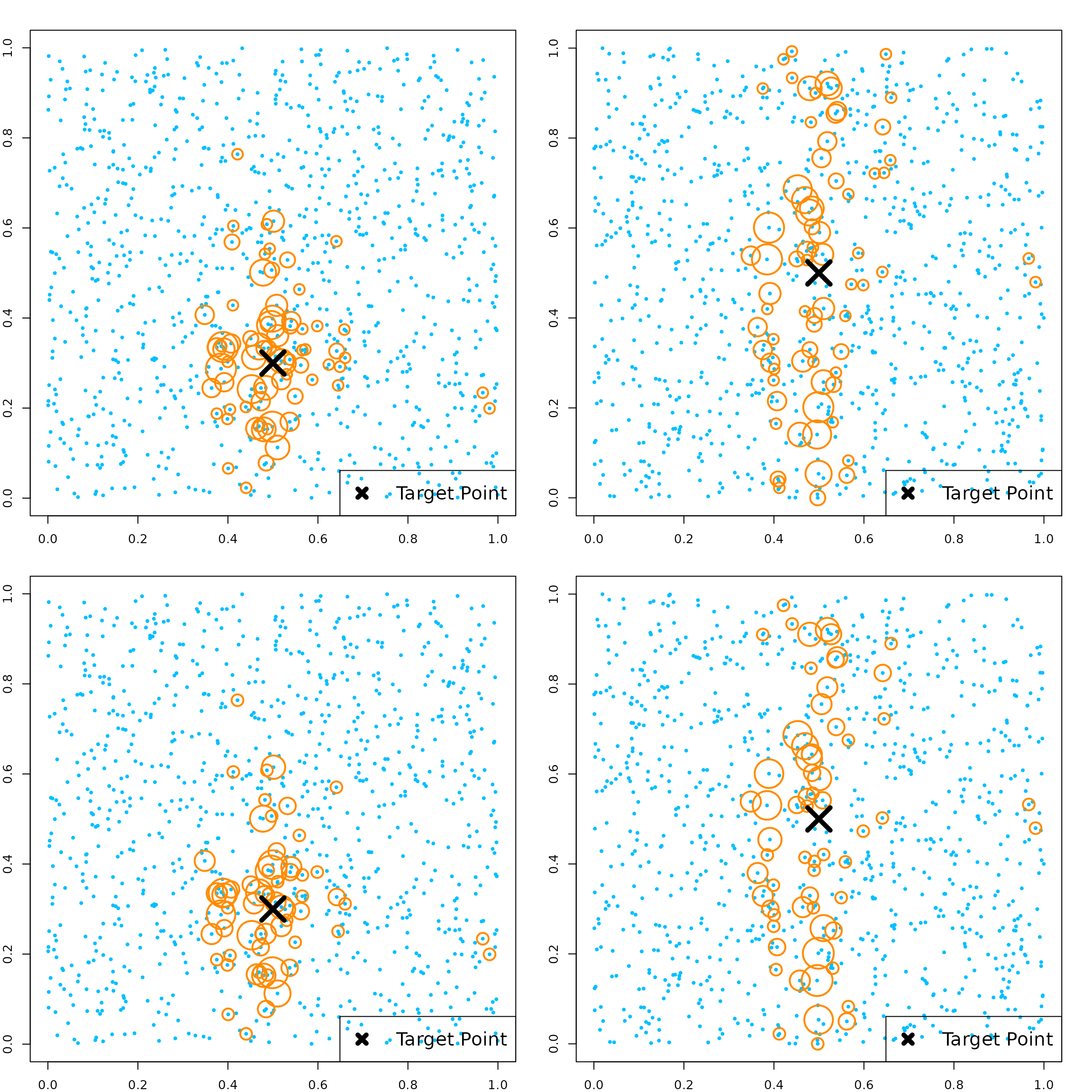
Setting random seed
  ## Fitting a forest
  RLTfit1 <- RLT(trainX, trainY, model = "regression",
                 ntrees = 100, importance = TRUE, nmin = 1)

  RLTfit2 <- RLT(trainX, trainY, model = "regression",
                 ntrees = 100, importance = TRUE, nmin = 1,
                 seed = RLTfit1$parameters$seed)

  # check if importance are identical
  all(RLTfit1$VarImp == RLTfit2$VarImp)
## [1] TRUE

  # prediction
  RLTPred1 <- predict(RLTfit1, testX, keep.all = TRUE)
  RLTPred2 <- predict(RLTfit2, testX, keep.all = TRUE)

  # check predictions are identical
  all(RLTPred1$Prediction == RLTPred2$Prediction)
## [1] TRUE