From a Penalized Objective to a Fitted Ridge Model

Optimization, tuning, and reliable implementation

← Week 3 overview · Review ridge theory · Next week: lasso and variable selection

The first ridge lecture explained why correlated predictors can make least-squares estimates unstable and how an $L_2$ penalty changes that behavior. We now turn the definition of ridge regression into a fitting procedure, study gradient descent in a setting where the exact answer is known, and choose the penalty by cross-validation or generalized cross-validation (GCV).

Learning goals

By the end of this lecture, you should be able to:

connect the ridge objective to its gradient, curvature matrix, and linear-system solution;
explain gradient descent in words and diagnose step sizes that are too small or too large;
distinguish solving ridge at a fixed penalty from choosing the penalty;
carry centering and standardization out separately inside every cross-validation training fold;
compute GCV from training error and effective degrees of freedom and compare its selected penalty with the cross-validation choice;
interpret a coefficient path, tuning curves, and a final test-set comparison; and
translate the course definition of $\lambda$ to common R and Python software conventions.

Optimize ridge for a fixed penalty

The ridge objective defines the fitted model for a chosen penalty. We now connect that objective to an exact solution and to an iterative algorithm that approaches the same minimum.

Why optimize a problem with a closed form?

Ridge regression has an explicit solution, so it is reasonable to ask why we should spend time on an iterative algorithm.

Ridge provides a clean setting for learning optimization because we already know the answer from an exact linear-system solve. We can watch an iterative method move toward that answer and ask concrete questions. Is each update moving downhill? Is the step size sensible? Has the algorithm reached the minimum?

These questions matter beyond ridge. The same ideas, including an objective function, gradient, curvature, step size, and stopping rule, reappear when a closed-form solution is unavailable.

Guiding question. How do we turn the mathematical definition of ridge regression into a reliable fitting-and-tuning procedure?

We will first solve one ridge objective in two ways, by a linear-system solve and by gradient descent. We will then choose the penalty using observations that were not used to fit each candidate model.

Keep three decisions separate:

Decision	Question it answers	Example in this lecture
Objective	What coefficient vector counts as a good fit for a fixed penalty?	Penalized squared error at a stated $\lambda$
Optimizer	How do we find the vector that minimizes that objective?	A linear-system solve or gradient descent
Tuning procedure	Which penalty should define the final fitting rule?	Cross-validation within the training set

Changing the optimizer should not change the fitted model when both algorithms accurately minimize the same objective. Changing $\lambda$ changes the objective itself. Cross-validation compares those different fitted rules.

Recap the ridge objective from Lecture 1

Lecture 1 derived the ridge solution, so we only recall the objects needed for optimization. Let $\mathbf X_{\mathrm{raw}}\in\mathbb R^{n\times p}$ contain the raw covariates. Training-sample means and scales transform it into the centered, standardized matrix $\mathbf X\in\mathbb R^{n\times p}$ . There are $p$ penalized slopes and $p+1$ total fitted coefficients after including the unpenalized intercept. With $\widetilde{\mathbf y}=\mathbf y-\bar y\mathbf 1_n$ and $\boldsymbol\beta\in\mathbb R^p$ , ridge minimizes

$L_\lambda(\boldsymbol\beta) = \frac{1}{2n}\lVert\widetilde{\mathbf y}-\mathbf X\boldsymbol\beta\rVert_2^2 +\frac{\lambda}{2}\lVert\boldsymbol\beta\rVert_2^2, \qquad \lambda\geq 0.$

The factors $1/2$ simplify differentiation, while $1/n$ fixes the numerical scale of $\lambda$ . To fit a model, compute preprocessing quantities from the available training rows, construct $\mathbf X$ and $\widetilde{\mathbf y}$ , solve for the $p$ standardized slopes, and then predict on the original response scale.

Preprocessing belongs to the fitted model

The means and scales are estimated quantities. Validation and test covariates must be transformed using values learned from the corresponding training rows. Computing them from the full dataset would allow those observations to affect the fitted model.

Gradient, curvature, and the linear-system solution

For reference, the gradient, curvature matrix, and normal equation from Lecture 1 are

$\begin{aligned} \nabla L_\lambda(\boldsymbol\beta) &= \frac{1}{n}\mathbf X^{\mathsf T}(\mathbf X\boldsymbol\beta-\widetilde{\mathbf y}) +\lambda\boldsymbol\beta,\\ \mathbf A_\lambda &= \frac{1}{n}\mathbf X^{\mathsf T}\mathbf X+\lambda\mathbf I_p,\\ \mathbf A_\lambda\widehat{\boldsymbol\beta}_\lambda &= \frac{1}{n}\mathbf X^{\mathsf T}\widetilde{\mathbf y}. \end{aligned}$

For $\lambda>0$ , $\mathbf A_\lambda$ is positive definite and the quadratic objective has one unique minimum. Numerical code should solve the last displayed linear system rather than construct a matrix inverse. The direct solve gives us a trusted comparison value for assessing gradient descent.

Gradient descent: follow the downhill direction

The gradient tells us how the objective changes near the current coefficient vector. Gradient descent moves in the opposite direction:

$\boldsymbol\beta^{(k+1)} = \boldsymbol\beta^{(k)} -\eta\nabla L_\lambda(\boldsymbol\beta^{(k)}),$

or, for ridge,

$\begin{aligned} \boldsymbol\beta^{(k+1)} &=\boldsymbol\beta^{(k)}\\ &\quad-\eta\left[ \frac{1}{n}\mathbf X^{\mathsf T} (\mathbf X\boldsymbol\beta^{(k)}-\widetilde{\mathbf y}) +\lambda\boldsymbol\beta^{(k)} \right]. \end{aligned}$

Here $\eta>0$ is the step size. A tiny step moves downhill but wastes iterations. A step that is too large can jump across the valley with increasing amplitude and never converge.

Curvature and step-size notation. Let $a_j$ be an eigenvalue of $\mathbf X^{\mathsf T}\mathbf X/n$ . The corresponding ridge curvature is $a_j+\lambda$ . If

$\mathbf e^{(k)} = \boldsymbol\beta^{(k)}-\widehat{\boldsymbol\beta}_\lambda,$

then the component of the optimization error in that eigendirection is multiplied at each update by

$1-\eta(a_j+\lambda).$

Let $m$ be the smallest eigenvalue of $\mathbf A_\lambda$ and let $M$ be its largest eigenvalue. The ratio $M/m$ is the condition number: a large ratio means a narrow, elongated quadratic valley, with much slower movement in low-curvature directions. Exact gradient descent converges from any starting value when every multiplier has absolute value below one, which is equivalent to

$\boxed{0<\eta<\frac{2}{M}}.$

The choice $\eta=1/M$ is a simple safe value for this example. It is not a universal rule. Practical optimizers may adapt the step as they run.

Before reading the code, keep these five steps in mind:

Input: a standardized design, centered response, penalty, initial coefficient vector, and step size.
Update: subtract the step size times the current gradient.
Store: retain the coefficient path, objective value, and gradient norm.
Stop: declare convergence only when the gradient norm is small, with a maximum-iteration safeguard.
Check: compare the final answer with the linear-system solution available for ridge.

The last step is especially important. An optimizer returning a coefficient vector is not evidence by itself that the vector minimizes the intended objective.

Watch three step sizes

We use the fixed six-predictor design and mean response from the ridge lecture. Each language generates one new response from that model when its code runs. R and Python use different random-number generators, so their realized responses and coefficient values need not match. We set $\lambda=0.2$ , start from the zero vector, and change only the step size within each language.

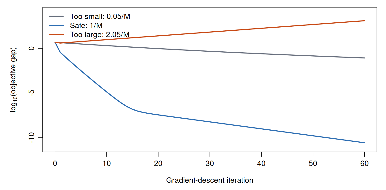
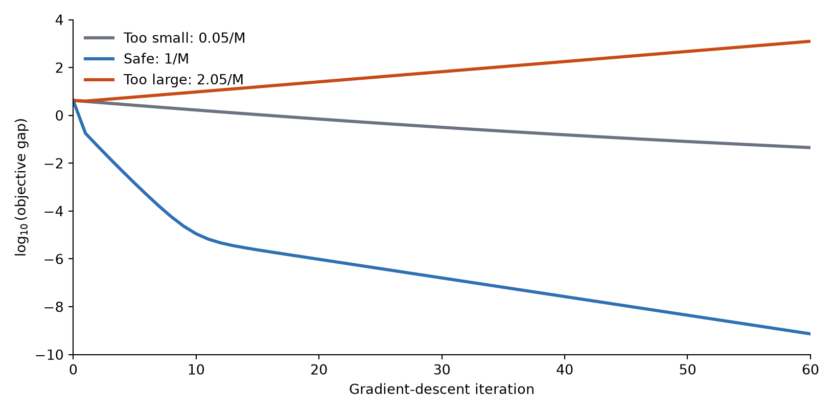
Predict the optimization paths. Compare the three steps before viewing the figure.

Too small: $\eta=0.05/M$ moves safely but slowly.
Safe: $\eta=1/M$ makes substantial progress without crossing the convergence boundary.
Too large: $\eta=2.05/M$ is just beyond $2/M$ . In this example, the current error has a component in the largest-curvature direction, and that component expands.

Which run should converge, which should converge slowly, and which should move away from the minimum?

Show the reproducible code

# Reuse the fixed design, then observe one new response for this demonstration.
fixed_demo_r <- read.csv("data/week-03/fixed-x.csv", check.names = FALSE)
feature_demo_r <- grep("^x[0-9]+$", names(fixed_demo_r), value = TRUE)
X_demo_raw_r <- as.matrix(fixed_demo_r[feature_demo_r])
set.seed(43232)
y_demo_raw_r <- fixed_demo_r$mu + rnorm(nrow(X_demo_raw_r))

Show the reproducible code

# Compute all centers and scales from the current training sample.

standardize_xy_r <- function(X_raw, y) {
  x_bar <- colMeans(X_raw)
  X_centered <- sweep(X_raw, 2, x_bar, "-")
  s <- sqrt(colMeans(X_centered^2))
  if (any(!is.finite(s)) || any(s <= 0)) {
    stop("Every predictor must have a positive finite training scale.")
  }
  list(
    X = sweep(X_centered, 2, s, "/"),
    y_centered = y - mean(y),
    x_bar = x_bar,
    s = s,
    y_bar = mean(y)
  )
}

ridge_closed_r <- function(X, y_centered, lambda) {
  p <- ncol(X)
  solve(crossprod(X) / nrow(X) + lambda * diag(p), crossprod(X, y_centered) / nrow(X))
}

ridge_objective_r <- function(beta, X, y_centered, lambda) {
  residual <- y_centered - drop(X %*% beta)
  sum(residual^2) / (2 * nrow(X)) + lambda * sum(beta^2) / 2
}

ridge_gradient_r <- function(beta, X, y_centered, lambda) {
  drop(crossprod(X, drop(X %*% beta) - y_centered) / nrow(X) + lambda * beta)
}

Show the reproducible code

# Use the direct solve to assess the gradient-descent result.

demo_r <- standardize_xy_r(X_demo_raw_r, y_demo_raw_r)
lambda_value <- 0.2
A_lambda <- crossprod(demo_r$X) / nrow(demo_r$X) +
  lambda_value * diag(ncol(demo_r$X))
curvatures <- eigen(
  A_lambda, symmetric = TRUE, only.values = TRUE
)$values
m <- min(curvatures)
M <- max(curvatures)
condition_number <- M / m
beta_closed <- ridge_closed_r(demo_r$X, demo_r$y_centered, lambda_value)
objective_star <- ridge_objective_r(
  beta_closed, demo_r$X, demo_r$y_centered, lambda_value
)

Show the reproducible code

# Start at zero and repeatedly subtract the gradient.
beta_hat <- rep(0, ncol(demo_r$X))
eta <- 1 / M

for (k in seq_len(20000)) {
  gradient <- drop(
    crossprod(
      demo_r$X,
      drop(demo_r$X %*% beta_hat) - demo_r$y_centered
    ) / nrow(demo_r$X) + lambda_value * beta_hat
  )

  if (sqrt(sum(gradient^2)) < 1e-10) {
    break
  }
  beta_hat <- beta_hat - eta * gradient
}

Three curves show objective gap by iteration. The small step decreases slowly, the safe step decreases quickly, and the step above the convergence boundary eventually increases. — Gradient-descent objective gap for three step sizes on the shared six-predictor ridge problem.

Gradient-descent verification against the closed-form solution
quantity	value
Smallest curvature m	2.005703e-01
Largest curvature M	2.337644e+00
Condition number M/m	1.165499e+01
Safe step 1/M	4.277811e-01
Iterations to gradient tolerance	1.760000e+02
Maximum coefficient difference	4.000000e-10

Show the reproducible code

# Reuse the fixed design, then observe one new response for this demonstration.
import numpy as np
import pandas as pd
import matplotlib.pyplot as plt

fixed_demo_py = pd.read_csv("data/week-03/fixed-x.csv")
feature_demo_py = [
    name for name in fixed_demo_py.columns
    if name.startswith("x") and name[1:].isdigit()
]
X_demo_raw_py = fixed_demo_py[feature_demo_py].to_numpy()
rng_demo_py = np.random.default_rng(43232)
y_demo_raw_py = (
    fixed_demo_py["mu"].to_numpy()
    + rng_demo_py.normal(size=X_demo_raw_py.shape[0])
)

Show the reproducible code

# Compute all centers and scales from the current training sample.

def standardize_xy_py(X_raw, y):
    x_bar = X_raw.mean(axis=0)
    s = np.sqrt(np.mean((X_raw - x_bar) ** 2, axis=0))
    if np.any(~np.isfinite(s)) or np.any(s <= 0):
        raise ValueError("Every predictor must have a positive finite training scale.")
    return {
        "X": (X_raw - x_bar) / s,
        "y_centered": y - y.mean(),
        "x_bar": x_bar,
        "s": s,
        "y_bar": y.mean(),
    }


def ridge_closed_py(X, y_centered, lam):
    p = X.shape[1]
    return np.linalg.solve(
        X.T @ X / X.shape[0] + lam * np.eye(p),
        X.T @ y_centered / X.shape[0],
    )


def ridge_objective_py(beta, X, y_centered, lam):
    residual = y_centered - X @ beta
    return (
        residual @ residual / (2 * X.shape[0])
        + lam * (beta @ beta) / 2
    )


def ridge_gradient_py(beta, X, y_centered, lam):
    return (
        X.T @ (X @ beta - y_centered) / X.shape[0]
        + lam * beta
    )

Show the reproducible code

# Use the direct solve to assess the gradient-descent result.

demo_py = standardize_xy_py(X_demo_raw_py, y_demo_raw_py)
lambda_value = 0.2
A_lambda = (
    demo_py["X"].T @ demo_py["X"] / demo_py["X"].shape[0]
    + lambda_value * np.eye(demo_py["X"].shape[1])
)
curvatures = np.linalg.eigvalsh(A_lambda)
m = curvatures.min()
M = curvatures.max()
condition_number = M / m
beta_closed = ridge_closed_py(
    demo_py["X"], demo_py["y_centered"], lambda_value
)
objective_star = ridge_objective_py(
    beta_closed, demo_py["X"], demo_py["y_centered"], lambda_value
)

Show the reproducible code

# Start at zero and repeatedly subtract the gradient.
beta_hat = np.zeros(demo_py["X"].shape[1])
eta = 1 / M

for k in range(20000):
    gradient = (
        demo_py["X"].T @ (demo_py["X"] @ beta_hat - demo_py["y_centered"])
        / demo_py["X"].shape[0]
        + lambda_value * beta_hat
    )

    if np.linalg.norm(gradient) < 1e-10:
        break
    beta_hat = beta_hat - eta * gradient

                           quantity         value
0              Smallest curvature m  2.005703e-01
1               Largest curvature M  2.337644e+00
2              Condition number M/m  1.165499e+01
3                     Safe step 1/M  4.277811e-01
4  Iterations to gradient tolerance  1.950000e+02
5    Maximum coefficient difference  3.333704e-10

The small step is not incorrect; it is inefficient. The large step is not simply noisy; it moves too far to converge. The safe run reaches the same coefficient vector as the linear-system solve, which checks the gradient formula and the stopping rule.

The objective defines the model

A linear-system solve and gradient descent are different algorithms for minimizing the same ridge objective. When they use the same data preparation and penalty convention and both are solved accurately, they should return the same fitted model up to numerical tolerance. An optimizer is not a different statistical method merely because its steps look different.

Choose and evaluate the penalty

Tuning asks a different question

Optimization holds $\lambda$ fixed and finds the coefficient vector that minimizes the objective. Tuning decides which value of $\lambda$ should be used. These are separate tasks.

Training error cannot answer the second question. At $\lambda=0$ , OLS minimizes training squared error over all coefficient vectors. Increasing $\lambda$ restricts the fit and can only make training RSS stay the same or increase. Ridge is useful only if the resulting reduction in variance improves prediction on responses that were not used for fitting.

We demonstrate the complete procedure with the diabetes data used in Week 2: 442 observations, ten baseline predictors, and a quantitative measure of disease progression one year later. We randomly assign 80% of the observations to a training set and the remaining 20% to a final test set. We then divide the training observations into ten folds. A fixed seed makes these assignments reproducible.

What the final test set is for

The test outcomes play no role in scaling, choosing $\lambda$ , or fitting the final coefficients. We inspect them once, after all choices have been made using the training data. The resulting test MSE is one assessment of the completed procedure on an untouched test set. It can be higher or lower than the procedure’s expected test performance because it is calculated from one particular test sample.

Ridge cross-validation, step by step

For each cross-validation fold and each candidate value of $\lambda$ :

use the other nine folds to compute predictor means, predictor scales, and the response mean;
standardize the fitting rows and transform the validation rows using those fitting-fold values;
solve ridge on the centered fitting response;
recover the intercept and predict the validation fold; and
record that fold’s mean squared error.

The ten fold errors are then summarized by

$\overline{\operatorname{MSE}}(\lambda) =\frac{1}{10}\sum_{k=1}^{10}\operatorname{MSE}_k(\lambda),$

and

$\operatorname{SE}(\lambda) = \frac{\operatorname{SD}\{\operatorname{MSE}_1(\lambda),\ldots, \operatorname{MSE}_{10}(\lambda)\}}{\sqrt{10}}.$

The cross-validation curve supports two common choices:

$\lambda_{\min}$ has the smallest mean cross-validation error.
$\lambda_{\mathrm{1se}}$ is the largest penalty whose mean error is no more than $\overline{\operatorname{MSE}}(\lambda_{\min})+\operatorname{SE}(\lambda_{\min})$ .

The one-standard-error rule accepts a somewhat larger estimated validation error in exchange for stronger shrinkage. “One standard error” refers to the conventional fold-to-fold variability summary displayed above. Because the ten fitted training sets overlap, their validation errors are dependent. Therefore $\operatorname{SE}(\lambda)$ is not a formal independent-sample standard error, and the one-standard-error rule is a model-selection heuristic rather than a confidence procedure.

LOOCV and generalized cross-validation

GCV provides a second training-only way to choose $\lambda$ . For each candidate penalty, fit ridge once on all training observations. If $\mathbf X$ is the standardized training matrix, the smoother including the unpenalized intercept is

$\mathbf H_\lambda = \frac{1}{n}\mathbf 1_n\mathbf 1_n^{\mathsf T} + \mathbf X \left( \mathbf X^{\mathsf T}\mathbf X+n\lambda\mathbf I_p \right)^{-1} \mathbf X^{\mathsf T}.$

For this fixed smoother, leave-one-out cross-validation (LOOCV) has the shortcut

$\operatorname{LOOCV}(\lambda) = \frac{1}{n}\sum_{i=1}^n \left\{ \frac{y_i-\widehat y_i} {1-(\mathbf H_\lambda)_{ii}} \right\}^2.$

GCV replaces the individual leverage values $(\mathbf H_\lambda)_{ii}$ by their average. The effective degrees of freedom are

$\operatorname{df}_{\mathrm{eff}}(\lambda) = \operatorname{tr}(\mathbf H_\lambda).$

At $\lambda=0$ and full column rank, $\operatorname{df}_{\mathrm{eff}}(0)=p+1$ . GCV adjusts the training MSE by this effective flexibility:

$\boxed{ \operatorname{GCV}(\lambda) = \frac{ n^{-1}\lVert(\mathbf I_n-\mathbf H_\lambda)\mathbf y\rVert_2^2 }{ \{1-\operatorname{df}_{\mathrm{eff}}(\lambda)/n\}^2 }. }$

For this calculation, predictor means and scales are estimated once from all training covariates and then held fixed along the penalty path. This differs from explicit fold-based cross-validation, which re-estimates preprocessing inside each training fold. The GCV shortcut treats the full-training smoother as fixed, so it does not represent that refitted preprocessing procedure exactly. GCV is a training-only tuning estimate, not an independent test result. We will compute it over exactly the same $\lambda$ grid used for ten-fold cross-validation and compare the selected penalties before examining the final test responses.

Create one common split and penalty grid

The following R chunk constructs the train-test split, the ten cross-validation folds, and the grid of candidate penalties. These objects are not part of the diabetes dataset. They are choices made for this analysis. We save them only so that the later Python code uses exactly the same observations, folds, and values of $\lambda$ .

Show the reproducible code

diabetes_shared <- read.csv(
  "data/week-02/diabetes.csv",
  check.names = FALSE
)

set.seed(43203)
n_total <- nrow(diabetes_shared)
n_test <- ceiling(0.20 * n_total)
test_index <- sample(seq_len(n_total), size = n_test)

split_shared <- rep("train", n_total)
split_shared[test_index] <- "test"
training_index <- which(split_shared == "train")

# Give the training observations approximately equal fold sizes.
fold_shared <- rep(NA_integer_, n_total)
fold_shared[training_index] <- sample(
  rep(seq_len(10), length.out = length(training_index))
)

split_folds_shared <- data.frame(
  row_id = seq_len(n_total),
  split = split_shared,
  cv_fold = fold_shared
)
lambda_grid_shared <- c(0, 10^seq(-4, 2, length.out = 61))

# These two files pass the same analysis choices to Python.
dir.create("data/week-03", recursive = TRUE, showWarnings = FALSE)
write.csv(
  split_folds_shared,
  "data/week-03/diabetes-split-folds.csv",
  row.names = FALSE
)
write.csv(
  data.frame(lambda = lambda_grid_shared),
  "data/week-03/diabetes-lambda-grid.csv",
  row.names = FALSE
)

table(split_folds_shared$split)


 test train 
   89   353

The split contains 353 training observations and 89 final test observations. From this point forward, both languages use the assignments and penalty grid generated above.

Recompute the complete training procedure

The code below implements the folds directly so that the location of every preprocessing step is visible. R and Python use the same observations, folds, and penalty grid, and they produce the same coefficient paths, fold errors, selected penalties, and test-set results.

Show the reproducible code

# Use the data, split, folds, and penalty grid generated above.
diabetes_r <- diabetes_shared
split_folds_r <- split_folds_shared
diabetes_r$row_id <- seq_len(nrow(diabetes_r))
diabetes_r <- merge(
  diabetes_r, split_folds_r,
  by = "row_id", all.x = TRUE, sort = FALSE
)
diabetes_r <- diabetes_r[order(diabetes_r$row_id), ]

feature_names_r <- setdiff(
  names(diabetes_r),
  c("row_id", "y", "split", "cv_fold")
)
lambda_grid_r <- lambda_grid_shared

train_rows_r <- diabetes_r$split == "train"
test_rows_r <- diabetes_r$split == "test"
X_train_raw_r <- as.matrix(diabetes_r[train_rows_r, feature_names_r])
y_train_raw_r <- diabetes_r$y[train_rows_r]
X_test_raw_r <- as.matrix(diabetes_r[test_rows_r, feature_names_r])
y_test_raw_r <- diabetes_r$y[test_rows_r]
fold_id_r <- diabetes_r$cv_fold[train_rows_r]

Show the reproducible code

# Fit ridge on one training sample and return coefficients on the original scale.

fit_ridge_model_r <- function(X_raw, y, lambda) {
  prepared <- standardize_xy_r(X_raw, y)
  beta_hat <- ridge_closed_r(prepared$X, prepared$y_centered, lambda)
  beta_hat_raw <- beta_hat / prepared$s
  raw_intercept <- prepared$y_bar - sum(prepared$x_bar * beta_hat_raw)

  list(
    beta_hat = beta_hat,
    beta_hat_raw = beta_hat_raw,
    raw_intercept = raw_intercept,
    x_bar = prepared$x_bar,
    s = prepared$s,
    y_bar = prepared$y_bar
  )
}

predict_ridge_r <- function(fit, X_new_raw) {
  drop(fit$raw_intercept + X_new_raw %*% fit$beta_hat_raw)
}

Show the reproducible code

# Refit preprocessing and ridge inside each cross-validation training sample.

fold_levels_r <- sort(unique(fold_id_r))
fold_mse_r <- matrix(
  NA_real_,
  nrow = length(fold_levels_r),
  ncol = length(lambda_grid_r)
)
validation_n_r <- integer(length(fold_levels_r))

for (k in seq_along(fold_levels_r)) {
  fold <- fold_levels_r[k]
  validation <- fold_id_r == fold
  validation_n_r[k] <- sum(validation)

  X_fold_raw <- X_train_raw_r[!validation, , drop = FALSE]
  y_fold <- y_train_raw_r[!validation]
  prepared <- standardize_xy_r(X_fold_raw, y_fold)
  X_validation <- sweep(
    X_train_raw_r[validation, , drop = FALSE],
    2, prepared$x_bar, "-"
  )
  X_validation <- sweep(X_validation, 2, prepared$s, "/")

  for (l in seq_along(lambda_grid_r)) {
    beta_hat <- ridge_closed_r(
      prepared$X,
      prepared$y_centered,
      lambda_grid_r[l]
    )
    y_hat <- prepared$y_bar + drop(X_validation %*% beta_hat)
    fold_mse_r[k, l] <-
      mean((y_train_raw_r[validation] - y_hat)^2)
  }
}

Show the reproducible code

# Apply the minimum-error and one-standard-error rules to the fold errors.

mean_cv_mse_r <- colMeans(fold_mse_r)
se_cv_mse_r <- apply(fold_mse_r, 2, sd) / sqrt(nrow(fold_mse_r))
minimum_index_r <- which.min(mean_cv_mse_r)
one_se_threshold_r <-
  mean_cv_mse_r[minimum_index_r] + se_cv_mse_r[minimum_index_r]
eligible_r <- which(mean_cv_mse_r <= one_se_threshold_r + 1e-12)
one_se_index_r <- eligible_r[which.max(lambda_grid_r[eligible_r])]
lambda_min_r <- lambda_grid_r[minimum_index_r]
lambda_1se_r <- lambda_grid_r[one_se_index_r]
gcv_curve_r <- ridge_path_r$train_mse /
  (1 - ridge_path_r$df_eff / nrow(X_train_raw_r))^2
gcv_index_r <- which.min(gcv_curve_r)
lambda_gcv_r <- lambda_grid_r[gcv_index_r]

cv_summary_r <- data.frame(
  lambda = lambda_grid_r,
  mean_cv_mse = mean_cv_mse_r,
  se_cv_mse = se_cv_mse_r,
  gcv = gcv_curve_r,
  one_se_threshold = rep(one_se_threshold_r, length(lambda_grid_r)),
  is_lambda_min = seq_along(lambda_grid_r) == minimum_index_r,
  is_lambda_1se = seq_along(lambda_grid_r) == one_se_index_r,
  is_lambda_gcv = seq_along(lambda_grid_r) == gcv_index_r
)

Show the reproducible code

# Use the same data, split, folds, and penalty grid generated above.
diabetes_py = pd.read_csv("data/week-02/diabetes.csv")
split_folds_py = pd.read_csv("data/week-03/diabetes-split-folds.csv")
diabetes_py.insert(0, "row_id", np.arange(1, len(diabetes_py) + 1))
diabetes_py = diabetes_py.merge(
    split_folds_py, on="row_id", how="left", validate="one_to_one"
).sort_values("row_id")

feature_names_py = [
    name for name in diabetes_py.columns
    if name not in {"row_id", "y", "split", "cv_fold"}
]
lambda_grid_py = pd.read_csv(
    "data/week-03/diabetes-lambda-grid.csv"
)["lambda"].to_numpy()

train_rows_py = diabetes_py["split"].eq("train").to_numpy()
test_rows_py = diabetes_py["split"].eq("test").to_numpy()
X_train_raw_py = diabetes_py.loc[train_rows_py, feature_names_py].to_numpy()
y_train_raw_py = diabetes_py.loc[train_rows_py, "y"].to_numpy()
X_test_raw_py = diabetes_py.loc[test_rows_py, feature_names_py].to_numpy()
y_test_raw_py = diabetes_py.loc[test_rows_py, "y"].to_numpy()
fold_id_py = diabetes_py.loc[train_rows_py, "cv_fold"].to_numpy(dtype=int)

Show the reproducible code

# Fit ridge on one training sample and return coefficients on the original scale.

def fit_ridge_model_py(X_raw, y, lam):
    prepared = standardize_xy_py(X_raw, y)
    beta_hat = ridge_closed_py(
        prepared["X"], prepared["y_centered"], lam
    )
    beta_hat_raw = beta_hat / prepared["s"]
    raw_intercept = prepared["y_bar"] - prepared["x_bar"] @ beta_hat_raw
    return {
        "beta_hat": beta_hat,
        "beta_hat_raw": beta_hat_raw,
        "raw_intercept": raw_intercept,
        "x_bar": prepared["x_bar"],
        "s": prepared["s"],
        "y_bar": prepared["y_bar"],
    }


def predict_ridge_py(fit, X_new_raw):
    return fit["raw_intercept"] + X_new_raw @ fit["beta_hat_raw"]

Show the reproducible code

# Refit preprocessing and ridge inside each cross-validation training sample.

fold_levels_py = np.sort(np.unique(fold_id_py))
fold_mse_py = np.empty((fold_levels_py.size, lambda_grid_py.size))
validation_n_py = np.empty(fold_levels_py.size, dtype=int)

for k, fold in enumerate(fold_levels_py):
    validation = fold_id_py == fold
    validation_n_py[k] = validation.sum()

    X_fold_raw = X_train_raw_py[~validation]
    y_fold = y_train_raw_py[~validation]
    prepared = standardize_xy_py(X_fold_raw, y_fold)
    X_validation = (
        X_train_raw_py[validation] - prepared["x_bar"]
    ) / prepared["s"]

    for l, lam in enumerate(lambda_grid_py):
        beta_hat = ridge_closed_py(
            prepared["X"],
            prepared["y_centered"],
            lam,
        )
        y_hat = prepared["y_bar"] + X_validation @ beta_hat
        fold_mse_py[k, l] = np.mean(
            (y_train_raw_py[validation] - y_hat) ** 2
        )

Show the reproducible code

# Apply the minimum-error and one-standard-error rules to the fold errors.

mean_cv_mse_py = fold_mse_py.mean(axis=0)
se_cv_mse_py = fold_mse_py.std(axis=0, ddof=1) / np.sqrt(fold_mse_py.shape[0])
minimum_index_py = int(np.argmin(mean_cv_mse_py))
one_se_threshold_py = (
    mean_cv_mse_py[minimum_index_py] + se_cv_mse_py[minimum_index_py]
)
eligible_py = np.flatnonzero(
    mean_cv_mse_py <= one_se_threshold_py + 1e-12
)
one_se_index_py = eligible_py[np.argmax(lambda_grid_py[eligible_py])]
lambda_min_py = lambda_grid_py[minimum_index_py]
lambda_1se_py = lambda_grid_py[one_se_index_py]
gcv_curve_py = (
    ridge_path_py["train_mse"]
    / (1 - ridge_path_py["df_eff"] / X_train_raw_py.shape[0]) ** 2
)
gcv_index_py = int(np.argmin(gcv_curve_py))
lambda_gcv_py = lambda_grid_py[gcv_index_py]

cv_summary_py = pd.DataFrame(
    {
        "lambda": lambda_grid_py,
        "mean_cv_mse": mean_cv_mse_py,
        "se_cv_mse": se_cv_mse_py,
        "gcv": gcv_curve_py,
        "one_se_threshold": one_se_threshold_py,
        "is_lambda_min": np.arange(lambda_grid_py.size) == minimum_index_py,
        "is_lambda_1se": np.arange(lambda_grid_py.size) == one_se_index_py,
        "is_lambda_gcv": np.arange(lambda_grid_py.size) == gcv_index_py,
    }
)

Read the coefficient path

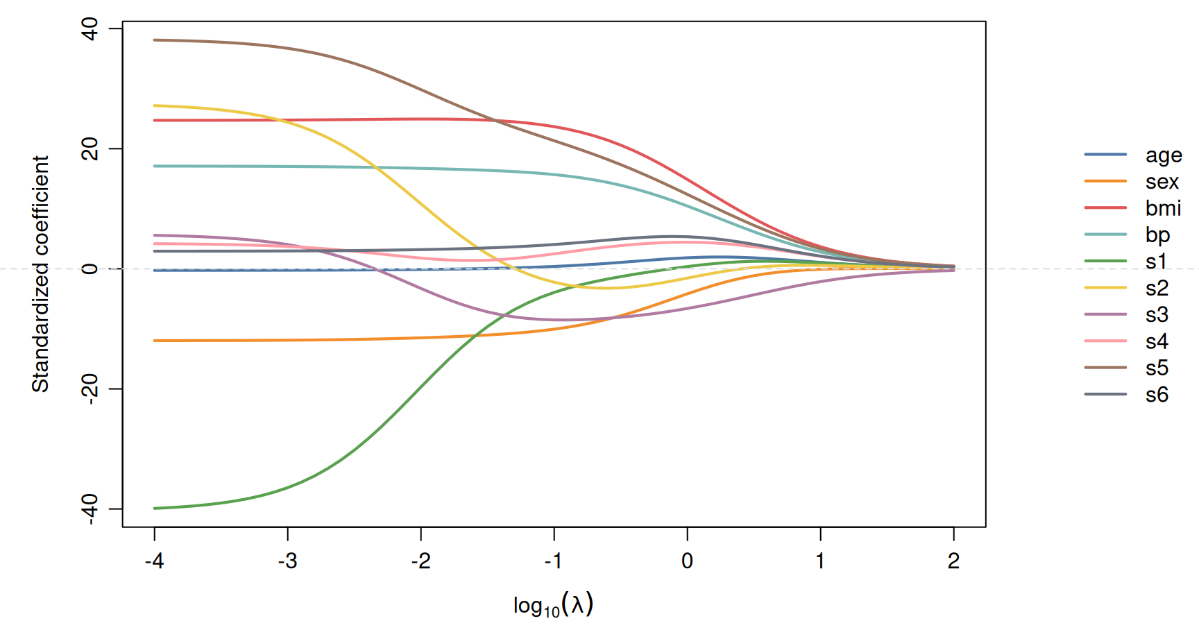
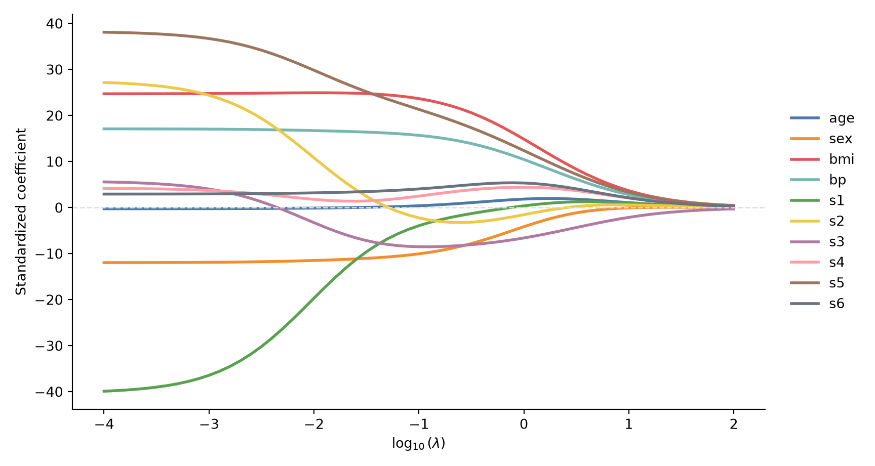
The coefficient path refits ridge on all 353 training rows over the common $\lambda$ grid. We plot coefficients on the standardized-predictor scale so that a one-unit change has the same scale meaning for every curve. Because the horizontal axis is $\log_{10}(\lambda)$ , this plot shows only the positive penalties. OLS is the limiting left endpoint and appears explicitly in the later tuning curve.

Ten coefficient curves move toward zero as log lambda increases. — Standardized ridge coefficient paths on the diabetes training split.

The curves change smoothly rather than jumping to zero. Ridge keeps every slope in the model but reduces their collective responsiveness to the data. Correlated serum measurements can also change sign or magnitude as their shared information is redistributed; a path is not a ranking of causal importance.

Compare the cross-validation and GCV curves

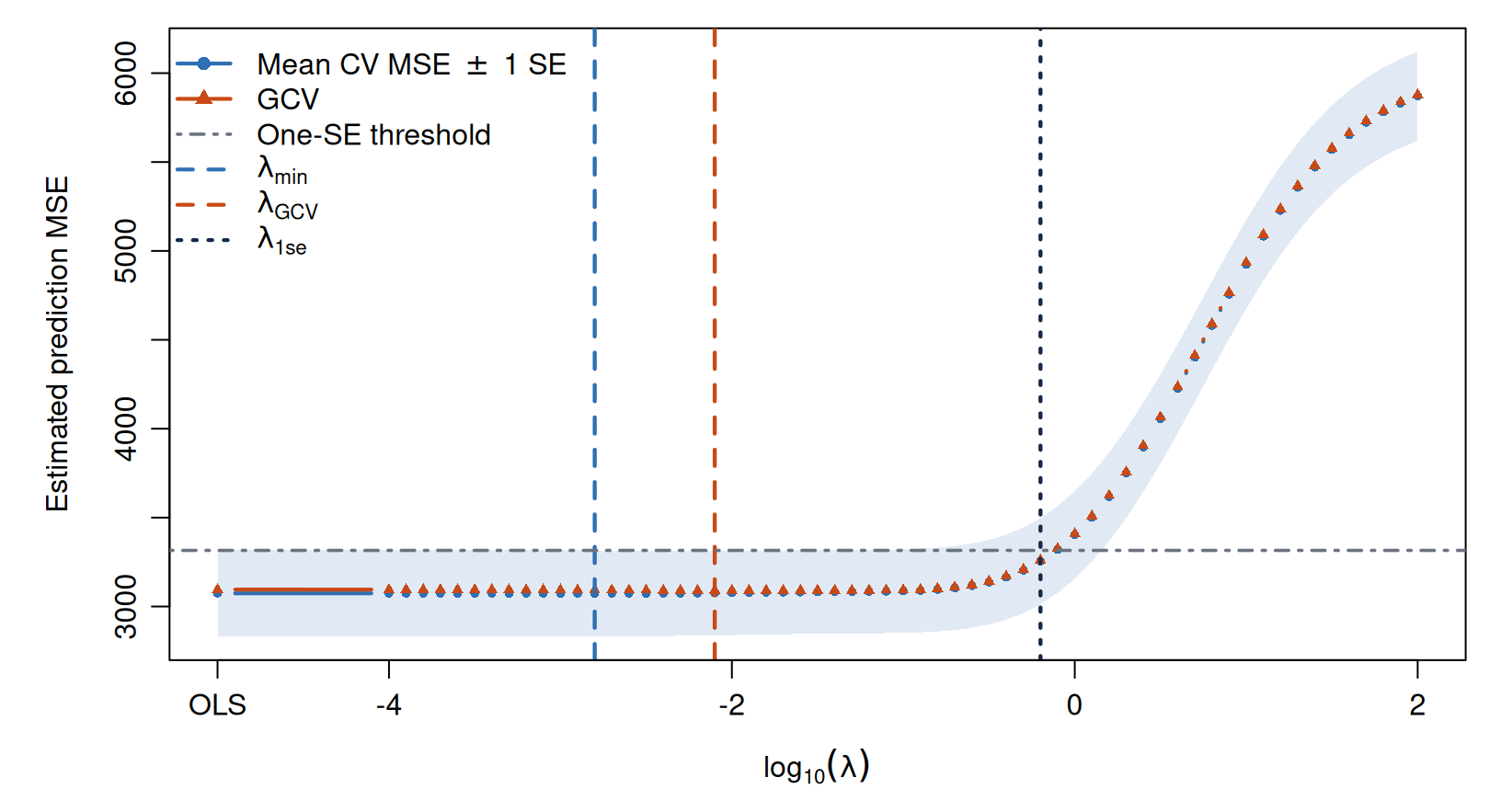
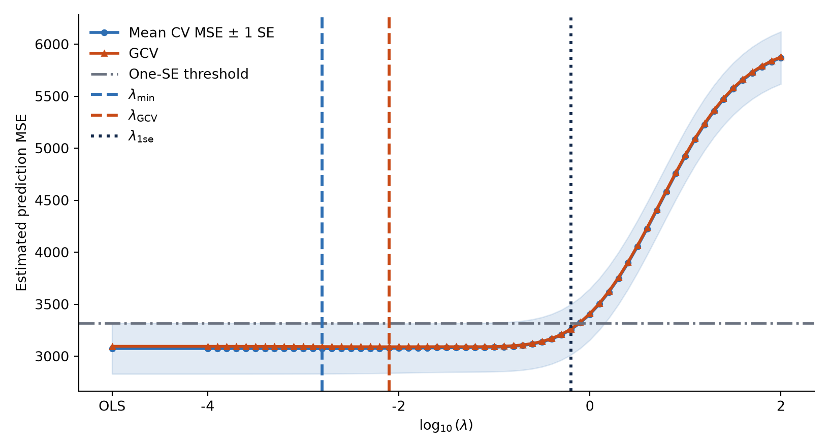
Both curves use the same candidate penalty grid. The cross-validation curve averages ten held-out-fold errors after refitting preprocessing within each fold. The GCV curve uses the full-training fit, its training MSE, and its effective degrees of freedom. The leftmost point represents OLS. Positive penalties are placed on a base-10 logarithmic scale; the OLS point is shown one plotting unit to the left of the smallest positive $\lambda$ .

Cross-validation and GCV error curves are plotted over the same lambda grid. Their minima occur at nearby but different penalties. A horizontal line and a third vertical line show the one-standard-error heuristic. — Ten-fold cross-validation and GCV estimates on the same ridge penalty grid. Vertical lines mark the CV minimum, one-standard-error, and GCV choices.

The cross-validation minimum occurs at $\lambda_{\min}=0.0016$ , with mean validation MSE $3073.49$ . The GCV curve reaches its minimum at $\lambda_{\mathrm{GCV}}=0.0079$ , so it chooses somewhat more shrinkage than the cross-validation minimum. The one-standard-error threshold is $3315.63$ , making the much larger value $\lambda_{\mathrm{1se}}=0.6310$ eligible under that heuristic. The choices need not agree: cross-validation repeatedly refits preprocessing on nine folds, while GCV evaluates one full-training linear smoother through its effective degrees of freedom.

Fix the choices and inspect the test set

After choosing the penalties, we refit each model on all 353 training rows and evaluate the untouched 89-row test set.

Show the reproducible code

# Report test error only after each tuning rule has selected its model.
heldout_display_r <- heldout_r[c(
  "model", "lambda", "df_eff", "train_mse", "test_mse"
)]
names(heldout_display_r) <- c(
  "Model", "Penalty lambda", "Effective df", "Training MSE", "Test MSE"
)
knitr::kable(
  heldout_display_r,
  digits = c(0, 4, 2, 1, 1),
  caption = "Training and test mean squared error"
)

Training and test mean squared error
Model	Penalty lambda	Effective df	Training MSE	Test MSE
OLS	0.0000	11.00	2905.4	2735.4
CV minimum	0.0016	10.82	2906.1	2731.7
One-SE	0.6310	5.79	3154.5	2925.2
GCV	0.0079	10.36	2911.9	2726.2

Show the reproducible code

# Report test error only after each tuning rule has selected its model.
heldout_py[
    ["model", "lambda", "df_eff", "train_mse", "test_mse"]
].rename(
    columns={
        "model": "Model",
        "lambda": "Penalty lambda",
        "df_eff": "Effective df",
        "train_mse": "Training MSE",
        "test_mse": "Test MSE",
    }
).round(
    {
        "Penalty lambda": 4,
        "Effective df": 2,
        "Training MSE": 1,
        "Test MSE": 1,
    }
)

        Model  Penalty lambda  Effective df  Training MSE  Test MSE
0         OLS          0.0000         11.00        2905.4    2735.4
1  CV minimum          0.0016         10.82        2906.1    2731.7
2      One-SE          0.6310          5.79        3154.5    2925.2
3         GCV          0.0079         10.36        2911.9    2726.2

OLS has the smallest training MSE, as it must. The cross-validation minimum and GCV choose modest shrinkage, with about $10.82$ and $10.36$ effective degrees of freedom, respectively. On this split, the GCV-selected fit has the smallest observed test MSE, $2726.2$ , followed closely by the cross-validation minimum at $2731.7$ . The one-standard-error heuristic chooses a much stronger penalty and has a larger observed test MSE here. These observations describe this test sample; they do not turn it into another tuning sample or prove that GCV has the smallest expected test error.

This table reports one observed test result, not the expected test performance of the four procedures. A different test sample could change the numerical values or even their ordering. The important design feature is that these 89 test outcomes were not used to choose $\lambda_{\min}$ , $\lambda_{\mathrm{1se}}$ , or $\lambda_{\mathrm{GCV}}$ .

Translate and interpret the fitted procedure

Translating the penalty across software

The name of a tuning argument is not enough to identify the fitted model. First write the objective, then map its constants.

Tool	Squared-error objective	Mapping from this lecture
This lecture	$\lVert\widetilde{\mathbf y}-\mathbf X\boldsymbol\beta\rVert^2/(2n)+\lambda\lVert\boldsymbol\beta\rVert^2/2$	$\lambda$
R `glmnet`, Gaussian family with `alpha = 0`	Same normalized objective	`lambda = lambda` after aligning centering, scaling, and intercept handling
Python `sklearn.linear_model.Ridge`	$\lVert\widetilde{\mathbf y}-\mathbf X\boldsymbol\beta\rVert^2+\alpha\lVert\boldsymbol\beta\rVert^2$	`alpha = n * lambda`

The mapping assumes that $\mathbf X$ and $\widetilde{\mathbf y}$ have already been constructed from the current training data and that the package does not center or standardize them again. Package defaults are convenient, but they must be included when stating which fitted model was used.

Limitations of the fitted procedure

Ridge can stabilize prediction when several variables carry overlapping information, but it does not make those variables uncorrelated and does not identify their separate causal effects. Its slopes are generally all nonzero, so it is not a variable-selection procedure. A fractional effective degrees of freedom measures the fitted values’ sensitivity to the observed responses; it is not a count of nonzero coefficients.

The test comparison comes from one split of a modest dataset. It demonstrates the correct order of operations: tune using the training data, fix all choices, and then evaluate on the test data. It does not prove that one penalty has smaller expected test error than OLS in every future sample. Repeated nested resampling would provide a fuller assessment of how much the result varies.

Review

Check your understanding

A gradient-descent step is $\eta=2.1/M$ . Why is this step too large for the quadratic objective considered here?
Why should gradient descent and the linear-system solve return the same coefficient vector when both are implemented correctly?
Why would standardizing all 442 rows before creating cross-validation folds leak information?
Ten-fold cross-validation and GCV choose different penalties on the same training data. Why is that difference not a contradiction?
Why is the GCV curve still a tuning estimate rather than an independent test evaluation?
Why might the observed test MSE ordering change if a different test sample were collected?

Key ideas

The ridge objective defines the fitted model; the optimizer is the method used to find its minimum.
For a fixed $\lambda>0$ , a linear-system solve and a correctly implemented gradient descent algorithm approach the same answer; the step size controls whether that iterative approach is efficient and stable.
Choosing $\lambda$ is a prediction problem, not an optimization problem. Training RSS alone always favors $\lambda=0$ .
Centering and scaling must be learned separately inside each cross-validation training fold.
GCV adjusts training error by the effective degrees of freedom of one full-training linear smoother; it can select a different penalty from fold-based cross-validation.
The one-standard-error rule is a conventional heuristic based on dependent fold errors. One final test MSE is an observed assessment, not an expected performance guarantee.

References and further reading

Golub, Heath, and Wahba (1979) introduced generalized cross-validation for choosing a ridge parameter.
James, Witten, Hastie, Tibshirani, and Taylor, An Introduction to Statistical Learning, Chapters 5 and 6, give accessible treatments of cross-validation and ridge regression.
Boyd and Vandenberghe, Convex Optimization provide a rigorous reference for convexity, optimality, and descent methods.
The official glmnet vignette and scikit-learn Ridge documentation state their objectives, preprocessing options, solvers, and cross-validation interfaces.