Skip to main content

Lasso and Sparsity

Theory and controlled computation

On this page

• Learning goals
• How lasso creates sparsity
• From the one-variable rule to a solution path
• Fitting, tuning, and comparing regularized models
• Interpreting a sparse fitted model
• Review

← Week 4 overview · Review ridge regression · Review optimization and cross-validation

Ridge regression stabilizes a fitted model by shrinking all slopes continuously toward zero. Lasso asks a different question: can regularization also produce a shorter fitted rule by setting some slopes exactly to zero? We begin with a one-variable calculation, use it to build a multivariable algorithm, and then examine what a sparse fit means when predictors are correlated.

Learning goals

By the end of this lecture, you should be able to:

• write the lasso objective using centered and standardized data;
• derive the one-variable soft-thresholding rule and explain why it can return exactly zero;
• explain how signal strength and the penalty affect selection across repeated samples;
• explain how coordinate descent and warm starts produce a lasso solution path;
• interpret a cross-validation curve without using the test set to choose the penalty; and
• compare the behavior of ridge, lasso, and elastic net when predictors are correlated.

How lasso creates sparsity

We begin with the limitation of ridge regression, define the lasso objective, and then use the one-variable problem to explain exact zeros and repeated selection.

Why ridge does not produce a sparse model

Ridge regression stabilizes a linear model by shrinking its slopes toward zero. It usually does not make them exactly zero. If a dataset has hundreds of predictors, a ridge fit will therefore usually contain hundreds of nonzero slopes, even when many of them are very small.

Sometimes we want a sparse model that uses only part of the available predictor set. The lasso replaces ridge’s squared-coefficient penalty with a sum of absolute values. This small change has an important consequence: for a range of penalty values, some fitted slopes are exactly zero.

Lasso still has the bias-variance trade-off from Week 3. Shrinkage introduces bias, but it can reduce sampling variation and improve prediction. The new feature is sparsity. Because prediction and recovery of the true variable set are different goals, we will use cross-validation to choose a predictive rule and interpret its nonzero coefficients cautiously.

Guiding question. What feature of the lasso penalty makes exact zeros possible, and what do those zeros mean when predictors are correlated?

We first answer this in a one-predictor problem. We then use the same calculation to understand selection across repeated samples, coordinate descent, a complete lasso path, and correlated predictors.

Define the lasso objective

Continue the ridge notation from Week 3. The matrix $\mathbf X$ again contains centered, standardized covariate columns, $\widetilde{\mathbf y}$ is the centered response, and the intercept is fitted separately. Ridge and lasso use the same data transformation. Only the penalty changes.

Let $\mathbf X_{\mathrm{raw}}\in\mathbb R^{n\times p}$ contain the covariates on their original scales, and let $\mathbf y\in\mathbb R^n$ contain the responses. Here $p$ is the number of slope covariates and $p+1$ is the total number of fitted coefficients after including the unpenalized intercept. As with ridge regression, the penalty should not depend on whether a variable is recorded in meters or millimeters. We therefore center and standardize each covariate using the current training data. Let $\mathbf X\in\mathbb R^{n\times p}$ denote the resulting matrix, and let

$$\widetilde{\mathbf y} = \mathbf y-\bar y\mathbf 1_n$$

be the centered response. Throughout this lecture, the lasso estimate is

$$\boxed{ \widehat{\boldsymbol\beta}_\lambda \in \operatorname*{arg\,min}_{\boldsymbol\beta\in\mathbb R^p} \left\{ \frac{1}{2n} \left\lVert \widetilde{\mathbf y}-\mathbf X\boldsymbol\beta \right\rVert_2^2 + \lambda\lVert\boldsymbol\beta\rVert_1 \right\}, \qquad \lambda\geq0. }$$

where

$$\lVert\boldsymbol\beta\rVert_1 = \sum_{j=1}^p|\beta_j|.$$

The optimization variable $\boldsymbol\beta$ contains the slopes on the standardized predictor scale. The squared-error term measures lack of fit. The penalty has the same value for positive and negative slopes of equal magnitude. The tuning parameter $\lambda$ determines how strongly we prefer smaller slopes.

• When $\lambda=0$, the objective reduces to least squares.
• As $\lambda$ increases, the slopes are pulled more strongly toward zero.
• The intercept is not penalized. After fitting the centered problem, it is recovered from the training means.

ImportantScaling is part of the fitted method

The centers and scales must be computed from the observations used to fit a model. During cross-validation, each validation fold is transformed using the centers and scales from the other folds. Computing them once from the full dataset would allow validation information to enter the fit.

The one-variable problem

The difference between ridge and lasso is easiest to see with one centered and standardized covariate $\mathbf x$, so that

$$\frac{1}{n}\mathbf x^{\mathsf T}\mathbf x=1.$$

Define

$$a=\frac{1}{n}\mathbf x^{\mathsf T}\widetilde{\mathbf y}.$$

In a one-predictor least-squares fit, $a$ is the fitted slope. Expanding the squared-error term gives

$$\begin{aligned} \frac{1}{2n} \left\lVert \widetilde{\mathbf y}-\mathbf x\beta \right\rVert_2^2 &= \frac{1}{2n} \widetilde{\mathbf y}^{\mathsf T}\widetilde{\mathbf y} - \beta\frac{\mathbf x^{\mathsf T}\widetilde{\mathbf y}}{n} + \frac{\beta^2}{2} \frac{\mathbf x^{\mathsf T}\mathbf x}{n}\\ &= \text{constant} + \frac{1}{2}(\beta-a)^2. \end{aligned}$$

Therefore, after removing terms that do not depend on $\beta$, the lasso objective becomes

$$\ell_\lambda(\beta) = \frac{1}{2}(\beta-a)^2+\lambda|\beta|.$$

The absolute-value term has a corner at zero, so we consider the two smooth sides separately.

If $\beta>0$, then $|\beta|=\beta$, and

$$\frac{d}{d\beta}\ell_\lambda(\beta) = \beta-a+\lambda.$$

Setting this derivative to zero gives $\beta=a-\lambda$. This answer lies on the positive side only when $a>\lambda$.

If $\beta<0$, then $|\beta|=-\beta$, and

$$\frac{d}{d\beta}\ell_\lambda(\beta) = \beta-a-\lambda.$$

The stationary point is now $\beta=a+\lambda$, and it lies on the negative side only when $a<-\lambda$.

What happens when $|a|\leq\lambda$? Immediately to the left of zero, the derivative is $-a-\lambda\leq0$. Immediately to the right, it is $-a+\lambda\geq0$. The objective decreases as it approaches zero from the left and increases after it passes zero. Its minimum is therefore exactly at zero.

Combining the three cases gives the soft-thresholding operator

$$S(a,\lambda) =\operatorname{sign}(a)(|a|-\lambda)_+ = \begin{cases} a-\lambda, & a>\lambda,\\ 0, & |a|\leq\lambda,\\ a+\lambda, & a<-\lambda. \end{cases}$$

Here $(u)_+=\max(u,0)$ denotes the positive part of $u$.

The fitted coefficient is not rounded to zero after optimization. Zero is the exact minimizer whenever the least-squares slope is no larger than the threshold in absolute value.

Compare ridge and lasso in one variable. Ridge gives $a/(1+\lambda)$, so a nonzero least-squares slope approaches zero smoothly. Lasso subtracts $\lambda$ from the slope’s absolute size and stops at zero. The corner of the absolute-value penalty creates this threshold.

WarningThe numerical value of the penalty depends on the objective

The threshold is $\lambda$ because the squared-error term is divided by $2n$. If a book or software package uses a different constant, the same fitted model may be labeled by a different numerical penalty. Compare the full objectives before comparing values of $\lambda$.

Watch the minimizer move

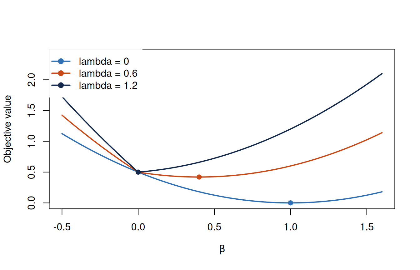
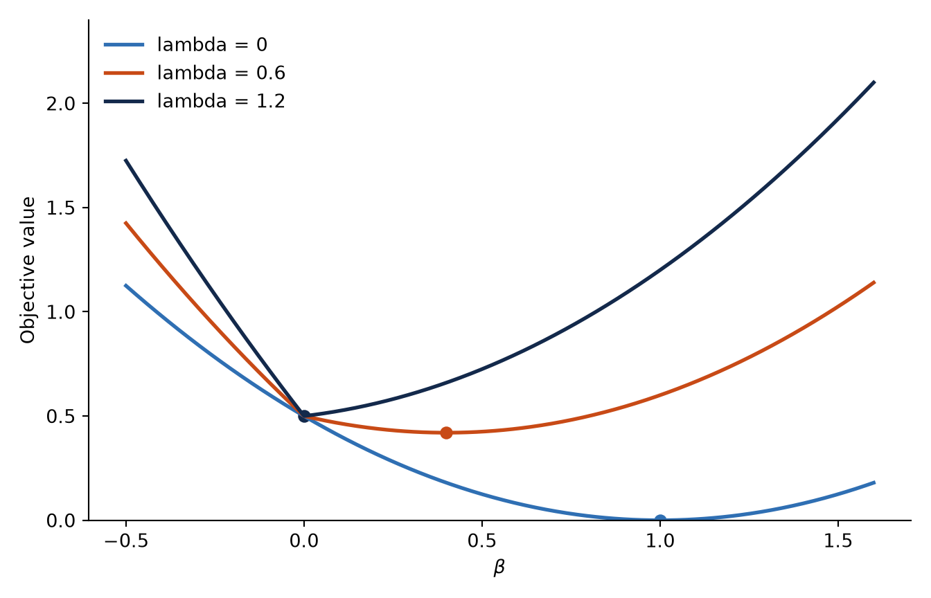
The next figure fixes the least-squares slope at $a=1$. Increasing $\lambda$ moves the minimizer toward zero. Once $\lambda\geq1$, zero becomes the exact minimizer.

R

# The corner in the absolute-value penalty moves the exact minimizer to zero.
a <- 1
beta_grid <- seq(-0.5, 1.6, length.out = 500)
lambda_values <- c(0, 0.6, 1.2)
curve_colors <- c("#2F6FB3", "#C84A16", "#13294B")

plot(
  NA,
  xlim = range(beta_grid), ylim = c(0, 2.4),
  xlab = expression(beta), ylab = "Objective value"
)
for (l in seq_along(lambda_values)) {
  lambda <- lambda_values[l]
  objective <- 0.5 * (beta_grid - a)^2 + lambda * abs(beta_grid)
  beta_hat <- sign(a) * max(abs(a) - lambda, 0)
  lines(beta_grid, objective, col = curve_colors[l], lwd = 2)
  points(
    beta_hat,
    0.5 * (beta_hat - a)^2 + lambda * abs(beta_hat),
    pch = 19, col = curve_colors[l]
  )
}
legend(
  "topleft", legend = paste("lambda =", lambda_values),
  col = curve_colors, lwd = 2, pch = 19, bty = "o",
  bg = "white", box.col = "white"
)

The one-variable lasso objective for three penalty values. The marked minimizer reaches zero once the penalty exceeds the absolute least-squares slope.

Python

import numpy as np
import matplotlib.pyplot as plt

# The corner in the absolute-value penalty moves the exact minimizer to zero.
a = 1
beta_grid = np.linspace(-0.5, 1.6, 500)
lambda_values = [0, 0.6, 1.2]
curve_colors = ["#2F6FB3", "#C84A16", "#13294B"]

fig, ax = plt.subplots(figsize=(7, 4.5))
for lam, color in zip(lambda_values, curve_colors):
    objective = 0.5 * (beta_grid - a) ** 2 + lam * np.abs(beta_grid)
    beta_hat = np.sign(a) * max(abs(a) - lam, 0)
    ax.plot(
        beta_grid,
        objective,
        color=color,
        linewidth=2,
        label=f"lambda = {lam}",
    )
    ax.scatter(
        beta_hat,
        0.5 * (beta_hat - a) ** 2 + lam * abs(beta_hat),
        color=color,
        s=35,
    )

ax.set(xlabel=r"$\beta$", ylabel="Objective value", ylim=(0, 2.4))
ax.legend(frameon=False)
ax.spines[["top", "right"]].set_visible(False)
fig.tight_layout()
plt.show()

The one-variable lasso objective for three penalty values. The marked minimizer reaches zero once the penalty exceeds the absolute least-squares slope.

The curves do not show a numerical rounding rule. They show a change in the location of the mathematical minimizer.

Decreasing signals and repeated selection

Soft thresholding explains why one fitted coefficient can equal zero. It does not imply that the same variables will be selected in every sample. The score $a_j$ depends on the response noise, so a variable near the threshold may be selected in one sample and omitted in another.

To isolate this effect, consider a fixed standardized design with $n=100$ observations and $p=20$ orthogonal covariates:

$$\frac{1}{n}\mathbf X^{\mathsf T}\mathbf X=\mathbf I_p.$$

Generate the response from

$$\mathbf y=\mathbf X\boldsymbol\beta+\boldsymbol\epsilon, \qquad \boldsymbol\epsilon\sim\mathcal N(\mathbf0,\mathbf I_n),$$

where every covariate has a nonzero coefficient, but the signal decreases with $j$:

$$\beta_j=0.4^{\sqrt j}, \qquad j=1,\ldots,p.$$

For this orthogonal design, the score for covariate $j$ satisfies

$$a_j = \frac{1}{n}\mathbf x_j^{\mathsf T}\mathbf y \sim \mathcal N\left(\beta_j,\frac{1}{n}\right),$$

and the fitted coefficient is

$$\widehat\beta_j(\lambda)=S(a_j,\lambda).$$

We independently repeat the response simulation 200 times. At each of three fixed penalties, we record whether each coefficient is nonzero and its absolute fitted magnitude. No new mathematical notation is needed for an individual run because every run applies the same calculation.

Because the distribution of each score has already been derived, we can generate the scores directly rather than reconstructing the full response vector in every repetition. The R and Python simulations use the same model and parameter values. Their exact draws differ because the two languages use different random-number generators.

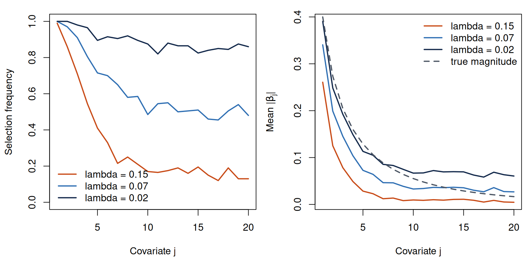
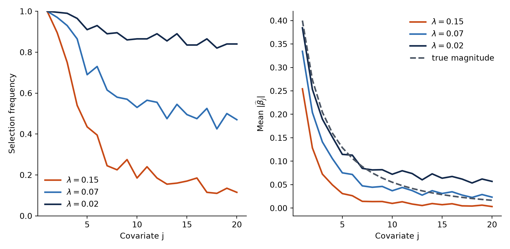
Predict the simulation before viewing it. Which covariates should be selected most often? What should happen to the selection frequencies and fitted magnitudes when $\lambda$ increases?

R

set.seed(43240)
n <- 100
p <- 20
n_simulations_r <- 200
beta <- 0.4^sqrt(seq_len(p))
lambda_values <- c(0.15, 0.07, 0.02)
curve_colors <- c("#C84A16", "#2F6FB3", "#13294B")

# Under orthogonality, each score has this normal distribution.
a_scores_r <- matrix(
  rnorm(
    n_simulations_r * p,
    mean = rep(beta, each = n_simulations_r),
    sd = 1 / sqrt(n)
  ),
  nrow = n_simulations_r,
  ncol = p
)
colnames(a_scores_r) <- paste0("a", seq_len(p))

# Dimensions are simulation, covariate, and penalty.
beta_hat_r <- array(
  0,
  dim = c(n_simulations_r, p, length(lambda_values))
)
for (l in seq_along(lambda_values)) {
  lambda <- lambda_values[l]
  beta_hat_r[, , l] <- sign(a_scores_r) * pmax(abs(a_scores_r) - lambda, 0)
}

selection_frequency_r <- apply(
  abs(beta_hat_r) > 1e-10,
  c(2, 3),
  mean
)
mean_magnitude_r <- apply(abs(beta_hat_r), c(2, 3), mean)

old_par_signal <- par(no.readonly = TRUE)
par(mfrow = c(1, 2), mar = c(4.2, 4.2, 1.2, 0.8))
matplot(
  seq_len(p), selection_frequency_r,
  type = "l", lty = 1, lwd = 2, col = curve_colors,
  ylim = c(0, 1), xlab = "Covariate j", ylab = "Selection frequency"
)
legend(
  "bottomleft", legend = paste("lambda =", lambda_values),
  col = curve_colors, lty = 1, lwd = 2, bty = "n"
)
matplot(
  seq_len(p), mean_magnitude_r,
  type = "l", lty = 1, lwd = 2, col = curve_colors,
  xlab = "Covariate j",
  ylab = expression("Mean " * "|" * hat(beta)[j] * "|")
)
lines(seq_len(p), beta, lty = 2, lwd = 2, col = "#4B5563")
legend(
  "topright",
  legend = c(paste("lambda =", lambda_values), "true magnitude"),
  col = c(curve_colors, "#4B5563"),
  lty = c(1, 1, 1, 2), lwd = 2, bty = "n"
)

Across 200 repetitions, stronger signals are selected more often. A larger penalty lowers both selection frequencies and average fitted magnitudes.

par(old_par_signal)

Python

import numpy as np
import matplotlib.pyplot as plt

rng = np.random.default_rng(43240)
n = 100
p = 20
n_simulations_py = 200
beta = 0.4 ** np.sqrt(np.arange(1, p + 1))
lambda_values = np.array([0.15, 0.07, 0.02])
curve_colors = ["#C84A16", "#2F6FB3", "#13294B"]

# Under orthogonality, each score has this normal distribution.
a_scores_py = rng.normal(
    loc=beta,
    scale=1 / np.sqrt(n),
    size=(n_simulations_py, p),
)

# Dimensions are simulation, covariate, and penalty.
beta_hat_py = np.stack(
    [
        np.sign(a_scores_py) * np.maximum(np.abs(a_scores_py) - lam, 0)
        for lam in lambda_values
    ],
    axis=2,
)
selection_frequency_py = (np.abs(beta_hat_py) > 1e-10).mean(axis=0)
mean_magnitude_py = np.abs(beta_hat_py).mean(axis=0)

fig, axes = plt.subplots(1, 2, figsize=(9, 4.4))
for l, (lam, color) in enumerate(zip(lambda_values, curve_colors)):
    axes[0].plot(
        np.arange(1, p + 1), selection_frequency_py[:, l],
        color=color, linewidth=2, label=fr"$\lambda={lam}$",
    )
    axes[1].plot(
        np.arange(1, p + 1), mean_magnitude_py[:, l],
        color=color, linewidth=2, label=fr"$\lambda={lam}$",
    )

axes[0].set(
    xlabel="Covariate j", ylabel="Selection frequency", ylim=(0, 1)
)
axes[1].plot(
    np.arange(1, p + 1), beta,
    color="#4B5563", linewidth=2, linestyle="--", label="true magnitude",
)
axes[1].set(xlabel="Covariate j", ylabel=r"Mean $|\widehat\beta_j|$")
for ax in axes:
    ax.legend(frameon=False)
    ax.spines[["top", "right"]].set_visible(False)
fig.tight_layout()
plt.show()

Across 200 repetitions, stronger signals are selected more often. A larger penalty lowers both selection frequencies and average fitted magnitudes.

The first covariates carry the strongest signals and are selected in nearly every repetition. Later covariates have smaller nonzero coefficients, so response noise more often moves their scores inside the interval $[-\lambda,\lambda]$. Increasing the penalty widens that interval, lowers selection frequencies, and shrinks the coefficients that remain nonzero.

This orthogonal-design benchmark isolates signal strength from competition among covariates. It gives us a clean reference point before returning to lasso geometry and the multivariable algorithm. The controlled example later in the lecture adds correlation, where two covariates can carry nearly the same predictive information and compete to represent it.

Different prediction targets can also favor different penalty values. At a target such as $\mathbf e_j$, the fitted conditional mean depends only on $\widehat\beta_j(\lambda)$. A strong coordinate may favor less shrinkage, while a weak coordinate may benefit from more variance reduction. Ordinary cross-validation still selects one penalty because it averages validation loss across the observed covariate distribution rather than optimizing prediction at one specially chosen target.

A geometric explanation

For every positive penalty, there is a corresponding constraint size $t\geq0$ for which the lasso solution also solves

$$\min_{\boldsymbol\beta} \left\lVert \widetilde{\mathbf y}-\mathbf X\boldsymbol\beta \right\rVert_2^2 \quad\text{subject to}\quad \lVert\boldsymbol\beta\rVert_1\leq t.$$

The factor $1/(2n)$ is omitted here because multiplying the constrained objective by a positive constant does not change its minimizer. The penalty value $\lambda$ and constraint size $t$ are not the same number. Their relationship depends on the observed data and need not be one-to-one when solutions are nonunique.

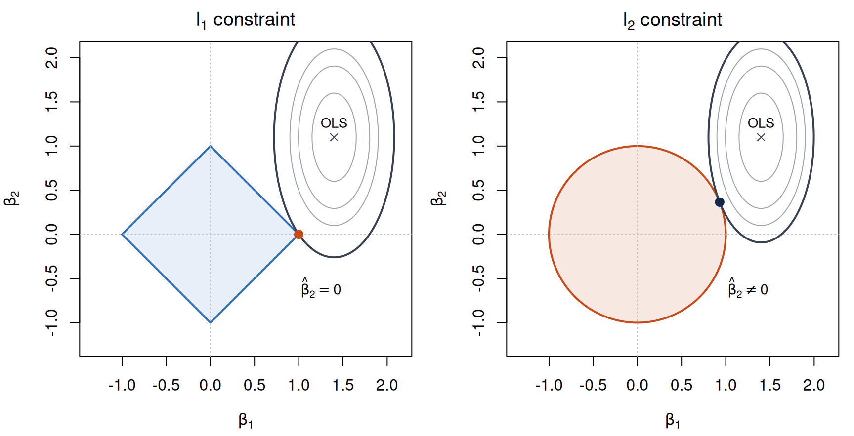
In two dimensions, the $\ell_1$ constraint is a diamond with corners on the coordinate axes. A least-squares contour can first touch the diamond at a corner, and a corner has one coordinate equal to zero. The ridge constraint is round, so first contact does not usually occur on an axis.

The same least-squares loss under L1 and L2 constraints. The bold ellipse is the first contour to touch each constraint. In this example, lasso touches the diamond at a corner with a zero second coefficient, while ridge touches the circle with both coefficients nonzero.

This picture helps explain why exact zeros are common, but the one-variable calculation gives the direct mathematical reason: an entire interval of scores is mapped to zero.

From the one-variable rule to a solution path

Coordinate descent and warm starts

With several covariates, the columns of $\mathbf X$ need not be orthogonal. Changing one slope changes the residual seen by the others, so the coefficients cannot generally be found by applying soft thresholding once to each separate least-squares slope.

Week 3 used gradient descent to move all ridge coefficients together in a downhill direction. Coordinate descent instead holds all but one coefficient fixed and solves the remaining one-variable lasso problem exactly. Both are algorithms for minimizing a fixed objective; neither chooses the penalty.

To update slope $j$, form the partial residual

$$\mathbf r_j = \widetilde{\mathbf y}-\sum_{k\ne j}\mathbf x_k\beta_k.$$

The corresponding one-variable score is

$$a_j = \frac{1}{n}\mathbf x_j^{\mathsf T}\mathbf r_j.$$

Because each standardized column satisfies $n^{-1}\mathbf x_j^{\mathsf T}\mathbf x_j=1$, the update is

$$\boxed{ \beta_j\leftarrow S(a_j,\lambda). }$$

After updating one coefficient, the algorithm moves to the next. It cycles through all predictors until the coefficients change by less than a chosen tolerance.

To calculate a full path, begin with a large penalty for which every slope is zero. Then decrease $\lambda$ and use the previous solution as the starting point for the next fit. This is called a warm start. Nearby penalty values usually have nearby solutions, so warm starts save substantial computation.

For standardized predictors, all slopes are zero whenever

$$\lambda \geq \lambda_{\max} = \left\lVert \frac{1}{n}\mathbf X^{\mathsf T}\widetilde{\mathbf y} \right\rVert_\infty.$$

The shared grid below starts at $1.7$. For the generated sample, this value exceeds $\lambda_{\max}$ for the full training sample and for every cross-validation training fold. Thus, every fitted path begins at the all-zero slope vector.

The lasso objective is convex, so exact convergence gives a global minimizer. A numerical stopping tolerance gives an approximation to that minimizer. Full column rank guarantees a unique coefficient vector. Rank deficiency permits, but does not require, multiple coefficient minimizers. Even when the coefficients are not unique, the fitted vector $\mathbf X\widehat{\boldsymbol\beta}_\lambda$ is unique. This is one reason to be cautious when interpreting which member of a correlated group is nonzero.

Stepwise and stagewise regression are different

Forward stepwise regression adds one predictor to the model in a full fitting step. Forward stagewise regression begins with all slopes at zero and repeatedly makes a small change to the coefficient that most reduces the current residual sum of squares. Because the residuals are reconsidered after every small move, a predictor can receive many updates along the path.

The lasso path is closely related to least-angle and forward-stagewise paths, which explains why variables appear gradually as the penalty decreases. These paths are not identical for every predictor configuration, and none of them should be interpreted as a universal ranking of variable importance. Coordinate descent is the computational method we use here because each update follows directly from the soft-thresholding calculation.

Fitting, tuning, and comparing regularized models

We now follow one controlled dataset from generation through fitting, cross-validation, and comparison with standard software.

A controlled example with correlated predictors

We now generate one dataset with 120 training observations, 80 final test observations, and eight predictors. The response has conditional mean

$$E(Y\mid\mathbf X_{\mathrm{raw}}) = 0.25+1.40X_{\mathrm{raw},1}-1.10X_{\mathrm{raw},3}+0.70X_{\mathrm{raw},5}.$$

Only $X_{\mathrm{raw},1}$, $X_{\mathrm{raw},3}$, and $X_{\mathrm{raw},5}$ appear in this data-generating mean. The error has a standard normal distribution. The raw predictors are generated so that $\operatorname{Cor}(X_{\mathrm{raw},1},X_{\mathrm{raw},2})=0.92$ and $\operatorname{Cor}(X_{\mathrm{raw},3},X_{\mathrm{raw},4})=0.75$ in the population.

The following chunk generates one realization. We use a separate seed for the fold assignments so that changing the response simulation later does not silently change the cross-validation folds. The saved CSV is only a bridge that lets the later Python chunk use exactly the same observations.

set.seed(43204)
n_train_r <- 120
n_test_r <- 80
p <- 8
n_r <- n_train_r + n_test_r

# Begin with independent standard normal variables.
independent_draws_r <- matrix(
  rnorm(n_r * p),
  nrow = n_r,
  ncol = p
)
X_raw_r <- independent_draws_r
X_raw_r[, 2] <- 0.92 * X_raw_r[, 1] +
  sqrt(1 - 0.92^2) * independent_draws_r[, 2]
X_raw_r[, 4] <- 0.75 * X_raw_r[, 3] +
  sqrt(1 - 0.75^2) * independent_draws_r[, 4]
X_raw_r[, 6] <- 3.5 * independent_draws_r[, 6]
colnames(X_raw_r) <- paste0("x", seq_len(p))

# Generate the response from the stated sparse regression model.
y_r <- 0.25 + 1.40 * X_raw_r[, 1] - 1.10 * X_raw_r[, 3] +
  0.70 * X_raw_r[, 5] + rnorm(n_r)

# Create five balanced folds among the training observations.
set.seed(43205)
fold_r <- rep(NA_integer_, n_r)
fold_r[seq_len(n_train_r)] <- sample(rep(1:5, each = n_train_r / 5))

lasso_data_r <- data.frame(
  row_id = seq_len(n_r),
  split = rep(c("train", "test"), c(n_train_r, n_test_r)),
  fold = fold_r,
  X_raw_r,
  y_reg = y_r,
  check.names = FALSE
)

dir.create("data/week-04", recursive = TRUE, showWarnings = FALSE)
write.csv(
  lasso_data_r,
  "data/week-04/lasso-simulation.csv",
  row.names = FALSE
)

training_rows_r <- lasso_data_r$split == "train"
round(c(
  `Cor(x1, x2)` = cor(lasso_data_r$x1[training_rows_r],
                       lasso_data_r$x2[training_rows_r]),
  `Cor(x3, x4)` = cor(lasso_data_r$x3[training_rows_r],
                       lasso_data_r$x4[training_rows_r])
), 3)

Cor(x1, x2) Cor(x3, x4) 
      0.897       0.780 

The sample correlations differ slightly from their population values because this is one random realization. Still, a correlated predictor can carry much of the same predictive information as a predictor that appears in the generating equation.

From this point forward, R and Python use the data generated above: the same response values, the same training and test split, the same five cross-validation folds, and the same decreasing grid of penalty values. Within each fit, the predictors are centered and standardized using only the observations available for training.

Predict the path before viewing it. As $\lambda$ moves from a large value toward zero, consider:

1. When should the first coefficients move away from zero?
2. Could $X_2$ or $X_4$ enter even though it does not appear in the generating equation?
3. If two fitted models keep different members of a correlated pair, must their test errors be very different?

Fit the shared path in R and Python

The following implementations show the coordinate update directly. Applied software uses the same basic idea together with additional computational shortcuts.

The objective uses standardized coefficients. To express the fitted model on the original predictor scale, use

$$\widehat\beta_{\mathrm{raw},j}=\frac{\widehat\beta_j}{s_j}, \qquad \widehat\beta_{0,\mathrm{raw}} =\bar y-\sum_{j=1}^p\bar x_j\widehat\beta_{\mathrm{raw},j}.$$

Thus the same prediction is $\bar y+\mathbf x^{\mathsf T}\widehat{\boldsymbol\beta}$ on standardized predictors or $\widehat\beta_{0,\mathrm{raw}}+\mathbf x_{\mathrm{raw}}^{\mathsf T}\widehat{\boldsymbol\beta}_{\mathrm{raw}}$ on raw predictors. The code uses beta_hat_raw when it retains the raw-scale coefficients.

R

# Use the data generated above and one fixed penalty.
features_r <- paste0("x", seq_len(p))
lambda_grid_r <- c(1.7, 1.5, 1.2, 0.8, 0.5, 0.3, 0.2, 0.12,
               0.08, 0.05, 0.03, 0.015)

train_r <- lasso_data_r$split == "train"
X_train_raw_r <- as.matrix(lasso_data_r[train_r, features_r])
y_train_r <- lasso_data_r$y_reg[train_r]
fold_r <- lasso_data_r$fold[train_r]

# Center and standardize using the training observations.
x_bar_r <- colMeans(X_train_raw_r)
s_r <- sqrt(colMeans(sweep(X_train_raw_r, 2, x_bar_r, "-")^2))
X <- sweep(
  sweep(X_train_raw_r, 2, x_bar_r, "-"),
  2,
  s_r,
  "/"
)
y_centered_r <- y_train_r - mean(y_train_r)

soft_threshold_r <- function(value, threshold) {
  sign(value) * pmax(abs(value) - threshold, 0)
}

# Each coordinate update is the one-variable soft-thresholding solution.
lambda_r <- 0.12
beta_hat_r <- rep(0, ncol(X))
for (k in 1:5000) {
  beta_old_r <- beta_hat_r
  for (j in seq_len(ncol(X))) {
    r_j <- y_centered_r -
      drop(X %*% beta_hat_r) +
      X[, j] * beta_hat_r[j]
    a_j <- mean(X[, j] * r_j)
    beta_hat_r[j] <- soft_threshold_r(a_j, lambda_r)
  }
  if (max(abs(beta_hat_r - beta_old_r)) < 1e-10) break
}

# Convert the standardized slopes back to the original predictor scale.
round(setNames(beta_hat_r / s_r, features_r), 3)

    x1     x2     x3     x4     x5     x6     x7     x8 
 1.113  0.003 -0.911  0.000  0.600  0.000  0.000  0.000 

rule	lambda	selected	CV_MSE	final_test_MSE
Minimum CV error	0.05	x1, x2, x3, x5, x6, x8	0.960	1.009
One standard error	0.12	x1, x2, x3, x5	0.983	1.053

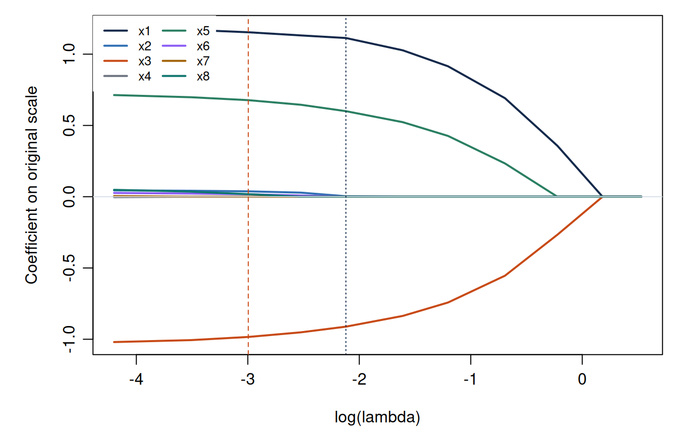
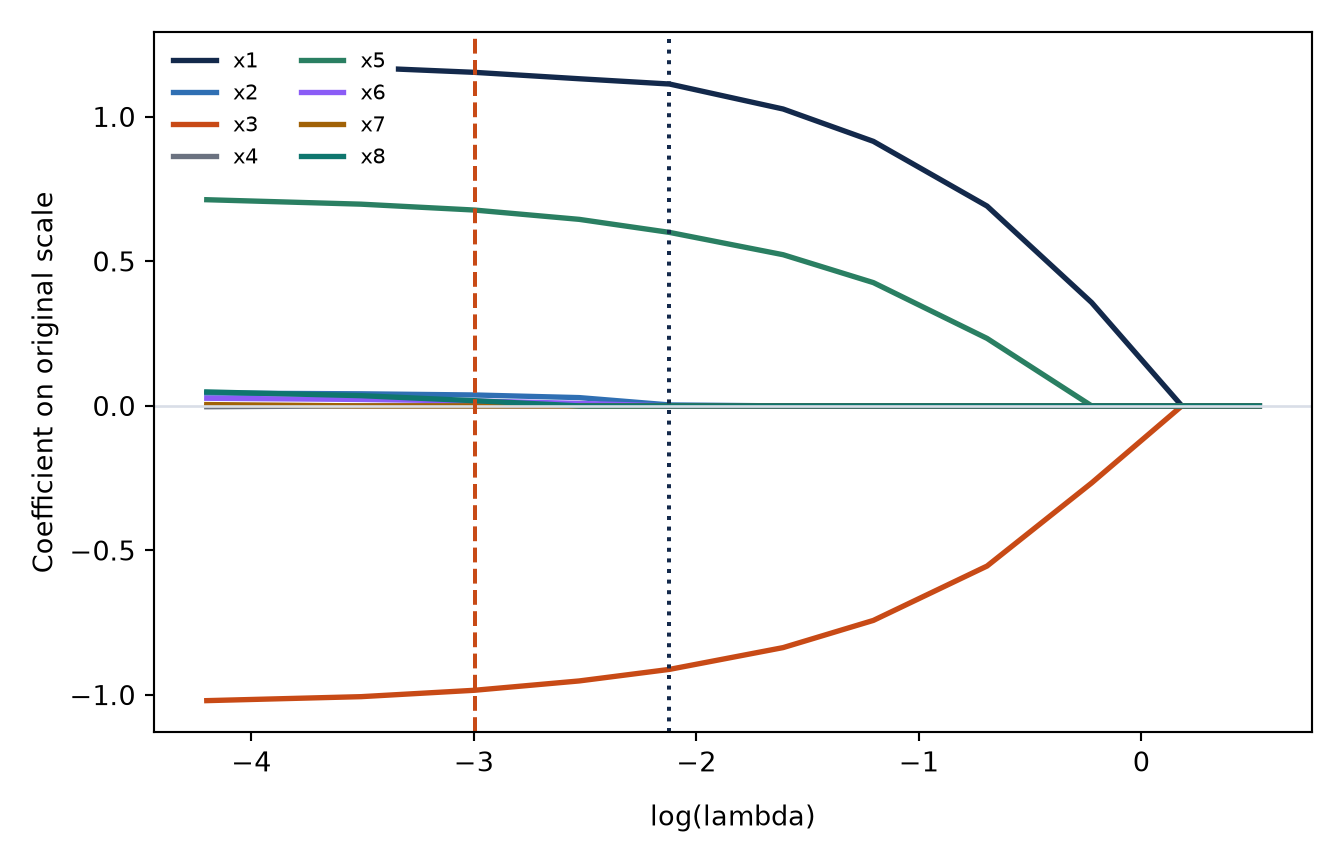
Lasso coefficient paths on the original predictor scale. The dashed orange line marks the minimum-error penalty, and the dotted navy line marks the one-standard-error penalty.

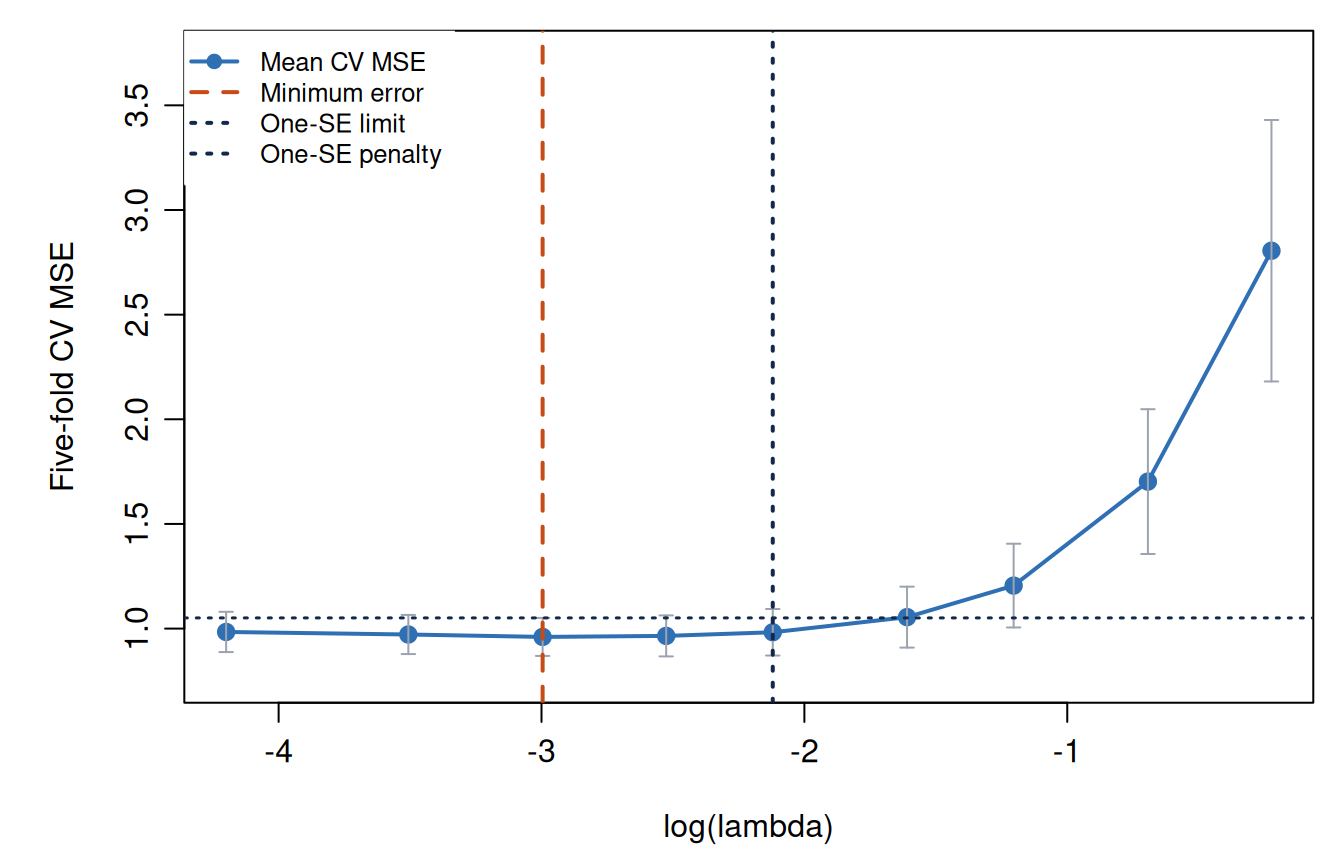
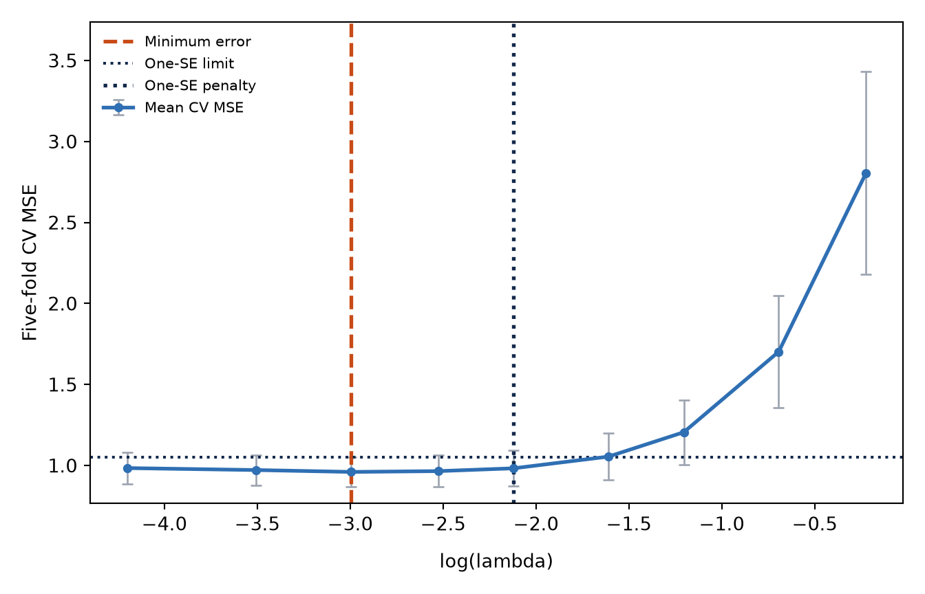
Five-fold cross-validation MSE along the lasso path. Error bars are one standard error across folds. The horizontal dotted line shows the one-standard-error limit.

Python

# Use the same observations generated and saved above.
import numpy as np
import pandas as pd
import matplotlib.pyplot as plt

lasso_data_py = pd.read_csv("data/week-04/lasso-simulation.csv")
p = 8
features_py = [f"x{j}" for j in range(1, p + 1)]
lambda_grid_py = np.array([
    1.7, 1.5, 1.2, 0.8, 0.5, 0.3, 0.2, 0.12,
    0.08, 0.05, 0.03, 0.015,
])

train_py = lasso_data_py["split"].eq("train").to_numpy()
X_train_raw_py = lasso_data_py.loc[train_py, features_py].to_numpy()
y_train_py = lasso_data_py.loc[train_py, "y_reg"].to_numpy()
fold_py = lasso_data_py.loc[train_py, "fold"].to_numpy()

# Center and standardize using the training observations.
x_bar_py = X_train_raw_py.mean(axis=0)
s_py = np.sqrt(((X_train_raw_py - x_bar_py) ** 2).mean(axis=0))
X = (X_train_raw_py - x_bar_py) / s_py
y_centered_py = y_train_py - y_train_py.mean()


def soft_threshold_py(value, threshold):
    return np.sign(value) * np.maximum(np.abs(value) - threshold, 0.0)


# Each coordinate update is the one-variable soft-thresholding solution.
lam = 0.12
beta_hat_py = np.zeros(X.shape[1])
for k in range(5000):
    beta_old_py = beta_hat_py.copy()
    for j in range(X.shape[1]):
        r_j = (
            y_centered_py
            - X @ beta_hat_py
            + X[:, j] * beta_hat_py[j]
        )
        a_j = np.mean(X[:, j] * r_j)
        beta_hat_py[j] = soft_threshold_py(a_j, lam)
    if np.max(np.abs(beta_hat_py - beta_old_py)) < 1e-10:
        break

# Convert the standardized slopes back to the original predictor scale.
print(pd.Series(beta_hat_py / s_py, index=features_py).round(3))

x1    1.113
x2    0.003
x3   -0.911
x4   -0.000
x5    0.600
x6    0.000
x7    0.000
x8    0.000
dtype: float64

              rule  lambda               selected  CV_MSE  final_test_MSE
  Minimum CV error    0.05 x1, x2, x3, x5, x6, x8   0.960           1.009
One standard error    0.12         x1, x2, x3, x5   0.983           1.053

Lasso coefficient paths on the original predictor scale. The dashed orange line marks the minimum-error penalty, and the dotted navy line marks the one-standard-error penalty.

<matplotlib.legend.Legend object at 0x7fa2e3c28510>

Five-fold cross-validation MSE along the lasso path. Error bars are one standard error across folds. The horizontal dotted line shows the one-standard-error limit.

Read the path and the cross-validation results

The algorithm computes the path from large penalties to small penalties so that it can use warm starts. The plotted horizontal axis increases from left to right, so small penalties appear on the left and large penalties appear on the right. At a sufficiently large $\lambda$, every slope is zero. As the penalty decreases, coefficients begin to move away from zero. Their paths need not move at the same rate because each coordinate update depends on the current residuals from all of the other predictors.

The path should not be read as a ranking of variable importance. In particular, a member of a correlated pair may enter because it carries information similar to the other member. A different response sample or a different set of folds can change which member enters first.

For each cross-validation fold, the code:

1. computes the predictor centers and scales from the other four folds;
2. fits every candidate penalty using those observations;
3. predicts the withheld fold; and
4. records the withheld-fold MSE.

The mean of the five fold MSEs estimates prediction performance for each penalty. The error bars use the standard deviation across folds divided by $\sqrt{5}$. We call this a fold-based standard-error estimate, not a formal confidence interval, because the fold fits use overlapping training observations. The estimated curve and its minimum can change when the data or fold assignment changes.

The complete path begins at $\lambda=1.7$. The cross-validation figure focuses on $\lambda\leq0.8$ because the larger penalties already show clear underfitting and would compress the differences near the minimum.

Two common choices summarize the curve:

• Minimum-error rule: choose the penalty with the smallest mean cross-validation MSE.
• One-standard-error rule: add the fold-based standard-error estimate at the minimum, then choose the largest penalty whose mean MSE is below that horizontal limit.

In this example, the minimum-error rule chooses $\lambda=0.05$ and retains $X_1$, $X_2$, $X_3$, $X_5$, $X_6$, and $X_8$. Predictor $X_2$ enters together with the signal-bearing predictor $X_1$, illustrating how correlated predictors can share a fitted contribution. The nonzero coefficients of $X_6$ and $X_8$ also remind us that selection in one sample does not prove that a variable belongs to the generating mean.

The one-standard-error rule chooses $\lambda=0.12$ and retains $X_1$, $X_2$, $X_3$, and $X_5$. It removes the two additional noise predictors but still keeps both members of the highly correlated pair $(X_1,X_2)$. Its validation error is slightly larger, but remains below the one-standard-error limit. The two selected fits have test MSEs $1.009$ and $1.053$. These are observed values from one test sample, so another test sample could change the values or their ordering. Different variable lists can still give similar predictions when the predictors contain overlapping information.

WarningThe test set is used after tuning

The test MSEs are reported only after the two cross-validation rules have been applied. If we inspected all test MSEs and chose the smallest one, the test rows would become part of the tuning process. The resulting test error would then be too favorable as an evaluation of the selected procedure.

Lasso, ridge, and elastic net

The three penalties express different preferences:

Method	Penalty term	Typical fitted pattern
Ridge	$\lambda\lVert\boldsymbol\beta\rVert_2^2/2$	Slopes shrink smoothly and are usually all nonzero. Correlated predictors often share the fitted contribution.
Lasso	$\lambda\lVert\boldsymbol\beta\rVert_1$	Some slopes are exactly zero. One member of a correlated group may represent information shared by the group.
Elastic net	$\lambda\{\alpha\lVert\boldsymbol\beta\rVert_1+(1-\alpha)\lVert\boldsymbol\beta\rVert_2^2/2\}$	The $\ell_1$ part can create zeros, while the $\ell_2$ part can make correlated coefficients move more stably together.

Here $0\leq\alpha\leq1$. Under this convention, $\alpha=1$ gives lasso and $\alpha=0$ gives ridge. Values between zero and one give elastic net. Both $\lambda$ and $\alpha$ must be chosen. If several values of $\alpha$ are compared, using the same cross-validation folds makes their estimated errors directly comparable.

For $\lambda>0$ and $\alpha<1$, the quadratic part makes the elastic-net coefficient solution unique. This is one reason elastic net can be more stable than lasso when predictors contain nearly the same information.

No penalty is uniformly best. Ridge is often useful when many predictors each contribute a little or when correlated predictors should be kept together. Lasso is useful when a shorter fitted rule is desired. Elastic net is a useful compromise when both sparsity and stability among correlated predictors matter.

Using standard software

The teaching code above makes the coordinate update visible. For an applied analysis, we normally use software that computes the path efficiently and checks convergence. The following examples preserve the training folds and place standardization inside the fitted procedure.

Write the objective before translating argument names:

Tool	Gaussian lasso objective	Course mapping
This lecture	$\lVert\widetilde{\mathbf y}-\mathbf X\boldsymbol\beta\rVert_2^2/(2n)+\lambda\lVert\boldsymbol\beta\rVert_1$	$\lambda$
R glmnet with alpha = 1	The same normalized form after its observation weights, intercept, and standardization conventions are matched	lambda = lambda
Python sklearn.linear_model.Lasso	$\lVert\widetilde{\mathbf y}-\mathbf X\boldsymbol\beta\rVert_2^2/(2n)+\mathtt{alpha}\lVert\boldsymbol\beta\rVert_1$	alpha = lambda

The alpha argument has different meanings in the two libraries. In glmnet, it mixes the lasso and ridge penalties. In scikit-learn’s Lasso, it is the penalty strength. Argument names are software choices, not mathematical notation.

R

# Match the package penalty scale to the course objective before tuning.
library(glmnet)

train <- subset(lasso_data_r, split == "train")
X_raw <- as.matrix(train[, features_r])
y <- train$y_reg

fit <- cv.glmnet(
  x = X_raw,
  y = y,
  family = "gaussian",
  alpha = 1,
  lambda = lambda_grid_r,
  foldid = train$fold,
  type.measure = "mse",
  standardize = TRUE
)


coef(fit, s = "lambda.min")
coef(fit, s = "lambda.1se")

Python

# This Pipeline fits standardization separately within every cross-validation fold.
from sklearn.linear_model import Lasso
from sklearn.model_selection import GridSearchCV
from sklearn.pipeline import Pipeline
from sklearn.preprocessing import StandardScaler

fold_splits = [
    (np.flatnonzero(fold_py != m), np.flatnonzero(fold_py == m))
    for m in range(1, 6)
]
pipeline = Pipeline([
    ("scale", StandardScaler()),
    ("lasso", Lasso(max_iter=20000, tol=1e-10)),
])
search = GridSearchCV(
    pipeline,
    param_grid={"lasso__alpha": lambda_grid_py},
    scoring="neg_mean_squared_error",
    cv=fold_splits,
    refit=True,
)
search.fit(X_train_raw_py, y_train_py)

# GridSearchCV chooses the smallest mean validation error.
search.best_params_

For Gaussian lasso, scikit-learn’s alpha plays the role of $\lambda$ in the objective used in this lecture. In glmnet, alpha = 1 requests lasso, while the argument lambda controls the penalty strength. The cv.glmnet() object reports both lambda.min and lambda.1se. GridSearchCV selects the minimum-error setting by default; applying a one-standard-error rule in Python requires reading the fold-level results and choosing the largest eligible penalty.

The name of an argument is not enough to establish that two fits are the same. Before comparing numerical penalty values, check the squared-error normalization, predictor standardization, response scaling, observation weights, and intercept treatment.

Interpreting a sparse fitted model

1. A zero coefficient is conditional on the other predictors and on $\lambda$. It means that this fitted rule did not use that predictor after accounting for the others at the chosen penalty.
2. A nonzero coefficient does not by itself establish scientific importance or a causal effect. Lasso is fitting a predictive relationship in the available data.
3. A stable prediction does not require a stable variable list. Correlated predictors can substitute for one another with little change in prediction error.
4. Large penalties can remove useful signal. Lasso reduces variation by adding shrinkage bias, just as ridge does.
5. Cross-validation does not reveal one fixed, universally best penalty. The selected value and the nonzero coefficients can change with the observed sample and fold assignment.

Review

Check your understanding

1. In the one-variable problem, why is the solution exactly zero when $|a|\leq\lambda$?
2. Why does ridge usually shrink a nonzero least-squares slope without making it exactly zero?
3. In coordinate descent, why must the partial residual be recomputed after other coefficients change?
4. In the decreasing-signal simulation, why can a truly nonzero coefficient have a selection frequency well below one?
5. Why can a correlated predictor be nonzero even when it does not appear in the generating equation for the controlled example?

Key ideas

1. Lasso uses an $\ell_1$ penalty and can produce an exactly sparse fitted coefficient vector.
2. Soft thresholding explains the exact zero: scores with absolute value no larger than $\lambda$ are mapped to zero.
3. Selection is sample-dependent. Stronger signals are selected more often, while a larger penalty lowers selection frequencies and fitted magnitudes.
4. Coordinate descent repeatedly solves one-variable problems, and warm starts make a full penalty path efficient.
5. Correlated predictors can give similar predictions while producing different lists of nonzero coefficients.
6. Cross-validation chooses a predictive rule, while the final test set evaluates it. Elastic net offers a compromise between lasso sparsity and ridge stability.

Looking ahead. Lasso selects among the original predictor coordinates. In Week 5, principal component analysis takes a different approach: it constructs new directions that summarize the predictor variation before a response model is fitted.

References and further reading

• Tibshirani, R. (1996), Regression Shrinkage and Selection via the Lasso.
• Zou, H. and Hastie, T. (2005), Regularization and Variable Selection via the Elastic Net.
• Friedman, J., Hastie, T., and Tibshirani, R. (2010), Regularization Paths for Generalized Linear Models via Coordinate Descent.
• James, Witten, Hastie, Tibshirani, and Taylor, An Introduction to Statistical Learning, Chapter 6, give an accessible discussion of ridge, lasso, and tuning.
• Hastie, Tibshirani, and Wainwright (2015), Statistical Learning with Sparsity, provide a more advanced treatment.
• Official implementation references: glmnet introduction, scikit-learn Lasso, and scikit-learn Pipeline.