Ridge Regression: Stability Through Shrinkage

Theory and fixed-design simulation

← Week 3 overview · Continue to optimization and cross-validation →

When covariates contain nearly the same information, ordinary least squares can fit the response well while its individual coefficient estimates change sharply from one sample to another. Ridge regression accepts some bias to reduce that instability. This lecture develops that idea from a correlated-covariate example and connects it to the bias-variance trade-off from Week 2.

Learning goals

By the end of this lecture, you should be able to:

explain why nearly redundant covariates make ordinary least squares unstable;
formulate ridge regression with slopes for standardized covariates and an unpenalized intercept;
derive its normal equation and closed-form solution;
interpret shrinkage for orthogonal covariates and for general principal directions;
explain in plain language how shrinkage trades squared bias for lower variance; and
connect ridge shrinkage to the effective-degrees-of-freedom idea from Week 2.

From instability to ridge regression

We begin with the instability caused by nearly redundant covariates, then ask how a penalty can stabilize their fitted coefficients.

Instability with correlated covariates

Ordinary least squares chooses the coefficient vector that fits the observed responses most closely. That sounds like an unqualified advantage. Why would we ever move away from its answer?

Imagine that two covariates record almost the same information. For example, two laboratory instruments may measure nearly the same biological quantity. The data can tell us that their combined contribution matters, but may contain very little information about how that contribution should be divided between the two coefficients. One sample may assign most of the effect to the first covariate; another sample may assign it to the second. Both fitted response vectors can be similar even while the individual coefficients move dramatically.

This is not mainly a story about an optimizer making a mistake. It is an information problem. The least-squares loss has a long, nearly flat valley: moving along the valley changes the coefficients substantially but changes the fitted values very little. Small changes in the response can therefore move the OLS solution a long distance.

Guiding question. Can we accept a small amount of bias in order to make coefficients and predictions much less sensitive to response noise?

Ridge regression answers yes. It shrinks the overall size of the slope vector. Its penalty adds curvature to weak directions, gives a unique solution when least squares is rank deficient, and reduces estimation variance. The cost is shrinkage bias.

Start with centered data

For now, suppose the covariate matrix $\mathbf X\in\mathbb R^{n\times p}$ already has column means zero and unit variances, and the response vector $\widetilde{\mathbf y}\in\mathbb R^n$ is already centered.¹ Here $n$ is the number of observations and $p$ is the number of covariates. The code calls the centered response y_centered.

The fitted intercept is zero on this centered scale, so we can concentrate on the $p$ slopes. The covariates can still be strongly correlated: putting them on a common scale does not remove the instability we want to study.

We will return to how to center and scale data, and recover coefficients in the original units after understanding the effect of shrinkage.

Define ridge regression

Let $\boldsymbol\beta\in\mathbb R^p$ contain the slopes for these standardized covariates. For a fixed penalty $\lambda\geq 0$ , ridge regression minimizes

$\boxed{ L_\lambda(\boldsymbol\beta) = \frac{1}{2n} \lVert\widetilde{\mathbf y}-\mathbf X\boldsymbol\beta\rVert_2^2 + \frac{\lambda}{2}\lVert\boldsymbol\beta\rVert_2^2. }$

The first term measures fit to the observed response. The second term penalizes large slopes. Its solution is

$\boxed{ \widehat{\boldsymbol\beta}_\lambda = \left(\mathbf X^{\mathsf T}\mathbf X+n\lambda\mathbf I_p\right)^{-1} \mathbf X^{\mathsf T}\widetilde{\mathbf y}. }$

We state the solution here so that we can use it in the simulation. We derive it after the simulation makes the stability problem visible.

At $\lambda=0$ , this reduces to OLS when $\mathbf X$ has full column rank. A positive $\lambda$ penalizes the size of the slope vector while leaving the intercept unpenalized. The rest of the lecture explains why this deliberate change can improve prediction.

A controlled experiment: stability under correlation

We hold one standardized covariate matrix fixed and repeatedly generate new response noise. The design has $n=80$ rows and $p=6$ covariates. To make the first two raw covariates nearly redundant, begin with independent standard normal variables and construct

$X_{\mathrm{raw},1}=L+0.025U_1, \qquad X_{\mathrm{raw},2}=L+0.025U_2,$

where $L$ , $U_1$ , and $U_2$ are independent. The remaining four raw covariates are independent standard normal variables. The setup code centers and scales these columns to produce the matrix $\mathbf X$ assumed above. The first two columns remain nearly redundant. We set

$\boldsymbol\beta = \begin{pmatrix} 1.5 & 1.5 & 1 & 0.75 & 0.5 & 0 \end{pmatrix}^{\mathsf T}, \qquad \boldsymbol\mu=\mathbf X\boldsymbol\beta, \qquad \sigma=1.$

Thus, the true mean depends on the sum of the first two covariates but not on their difference.

Each repetition uses the same covariates and the same true mean. Only the random response noise changes. Each repetition also includes a second, independent response at those same covariate values so that we can ask how well a fitted model predicts a response it did not see.

This is fixed-design prediction. The independent response changes the noise while keeping the covariate rows fixed, so it isolates the effect of response noise. It does not evaluate prediction at newly sampled covariate values.

Predict before calculation.

Will the two OLS slopes be stable when the response noise changes?
Will their sum be more stable than either slope separately?
If ridge makes the slopes less variable, must it also improve prediction?

In one repetition, the observed response and an independent test response are

$\begin{aligned} \mathbf y&=\boldsymbol\mu+\boldsymbol\epsilon,\\ \mathbf y^*&=\boldsymbol\mu+\boldsymbol\epsilon^*, \end{aligned}$

where

$E(\boldsymbol\epsilon\mid\mathbf X) = E(\boldsymbol\epsilon^*\mid\mathbf X) =\mathbf 0, \qquad \operatorname{Cov}(\boldsymbol\epsilon\mid\mathbf X) = \operatorname{Cov}(\boldsymbol\epsilon^*\mid\mathbf X) =\sigma^2\mathbf I_n.$

The two error vectors are independent and have normal distributions. We repeat this experiment independently 1,000 times while keeping $\mathbf X$ and $\boldsymbol\mu$ fixed.

Each generated response $\mathbf y$ can have a nonzero sample mean $\bar y$ . The code subtracts that mean to obtain $\widetilde{\mathbf y}$ for fitting the slopes, then adds it back for prediction. This fits $p$ slopes and one unpenalized intercept, for $p+1$ mean coefficients in total.

We highlight OLS, $\lambda=0$ , and two positive penalties. Within one repetition, every penalty is fitted to the same realized training response and evaluated on the same realized independent test response. Only after all penalties have been compared do we draw a new response pair for the next repetition.

The following R chunk generates and saves the fixed covariates and their true mean response. R and Python then run separate seeded simulations, drawing fresh errors inside each repetition. Their Monte Carlo results need not match numerically, but both should track the same theoretical expectations.

Show the reproducible code

set.seed(43203)
n <- 80
p <- 6
repetitions <- 1000
sigma <- 1

# Make the first two raw covariates nearly redundant.
L <- rnorm(n)
U1 <- rnorm(n)
U2 <- rnorm(n)
X_raw <- cbind(
  x1 = L + 0.025 * U1,
  x2 = L + 0.025 * U2,
  x3 = rnorm(n),
  x4 = rnorm(n),
  x5 = rnorm(n),
  x6 = rnorm(n)
)

feature_names <- colnames(X_raw)

# Center each covariate so its average squared value is one.
x_bar <- colMeans(X_raw)
X <- sweep(X_raw, 2, x_bar, "-")
s <- sqrt(colMeans(X^2))
X <- sweep(X, 2, s, "/")

beta <- c(1.5, 1.5, 1, 0.75, 0.5, 0)
mu <- drop(X %*% beta)

# Save the genuine raw covariates. Each language then performs the stated
# centering and standardization before fitting.
ridge_data <- data.frame(
  row_id = seq_len(n), X_raw, mu = mu, check.names = FALSE
)

dir.create("data/week-03", recursive = TRUE, showWarnings = FALSE)
write.csv(
  ridge_data, "data/week-03/fixed-x.csv", row.names = FALSE
)

singular_values <- svd(X, nu = 0, nv = 0)$d
round(c(
  "Cor(x1, x2)" = cor(X[, 1], X[, 2]),
  `Largest singular value` = max(singular_values),
  `Smallest singular value` = min(singular_values),
  `Condition number` = (max(singular_values) / min(singular_values))^2
), 3)

            Cor(x1, x2)  Largest singular value Smallest singular value 
                  0.999                  13.077                   0.214 
       Condition number 
               3748.488

In this realized design, $\operatorname{Cor}(\mathbf x_1,\mathbf x_2)=0.99931$ . The largest and smallest singular values of $\mathbf X$ are approximately $13.077$ and $0.214$ , so the unpenalized quadratic loss has condition number about $3748.5$ . For this quadratic loss, the condition number is the largest curvature eigenvalue divided by the smallest. A large ratio means that some coefficient directions are much flatter than others. The correlation, singular values, and loss geometry all express the same point: the two columns are nearly copies, the difference direction is barely visible, and the least-squares loss is extremely elongated.

A direct simulation in R and Python

Show the reproducible code

lambda_values <- c(0, 0.02, 0.2)
lambda_grid_r <- c(
  0, 0.0001, 0.0002, 0.0005, 0.001, 0.002, 0.005,
  0.01, 0.02, 0.05, 0.1, 0.2, 0.5, 1, 2, 5, 10
)
gram <- crossprod(X)

# Repeat the experiment. New noise is drawn only when a run begins.
train_mse_draws_r <- matrix(
  NA_real_, nrow = repetitions, ncol = length(lambda_grid_r)
)
test_mse_draws_r <- matrix(
  NA_real_, nrow = repetitions, ncol = length(lambda_grid_r)
)
# Axes index repetitions, coefficients, and penalties.
beta_hat <- array(
  NA_real_, dim = c(repetitions, p, length(lambda_grid_r))
)
intercept_draws_r <- numeric(repetitions)
selected_grid_positions <- match(lambda_values, lambda_grid_r)

set.seed(43205)
for (k in seq_len(repetitions)) {
  train_error <- rnorm(n, sd = sigma)
  test_error <- rnorm(n, sd = sigma)
  y_train <- mu + train_error
  y_test <- mu + test_error
  y_bar <- mean(y_train)
  y_centered <- y_train - y_bar
  intercept_draws_r[k] <- y_bar

  # Reuse this run's realized training/test pair across all penalties.
  for (l in seq_along(lambda_grid_r)) {
    lambda <- lambda_grid_r[l]
    beta_hat[k, , l] <- solve(
      gram + n * lambda * diag(p),
      crossprod(X, y_centered)
    )
    y_hat <- y_bar + drop(X %*% beta_hat[k, , l])

    train_mse_draws_r[k, l] <- mean((y_train - y_hat)^2)
    test_mse_draws_r[k, l] <- mean((y_test - y_hat)^2)

  }
}

knitr::kable(
  data.frame(
    lambda = lambda_values,
    beta_1 = beta_hat[repetitions, 1, selected_grid_positions],
    beta_2 = beta_hat[repetitions, 2, selected_grid_positions],
    train_mse = train_mse_draws_r[repetitions, selected_grid_positions],
    test_mse = test_mse_draws_r[repetitions, selected_grid_positions]
  ),
  digits = c(3, 3, 3, 3, 3),
  caption = "One realized training/test response pair"
)

One realized training/test response pair
lambda	beta_1	beta_2	train_mse	test_mse
0.00	-2.010	5.391	0.835	1.151
0.02	1.565	1.783	0.852	1.121
0.20	1.507	1.539	1.017	1.129

Show the reproducible code

import numpy as np
import pandas as pd
import matplotlib.pyplot as plt

# Read the fixed raw design generated above, then apply the same
# centering and standardization used in R.
ridge_data = pd.read_csv("data/week-03/fixed-x.csv")
feature_names = [
    name for name in ridge_data.columns
    if name.startswith("x") and name[1:].isdigit()
]
X_raw = ridge_data[feature_names].to_numpy()
x_bar = X_raw.mean(axis=0)
X_centered = X_raw - x_bar
s = np.sqrt(np.mean(X_centered**2, axis=0))
X = X_centered / s
mu = ridge_data["mu"].to_numpy()
beta = np.array([1.5, 1.5, 1, 0.75, 0.5, 0])

n, p = X.shape
repetitions = 1000
sigma = 1.0
lambda_values = np.array([0.0, 0.02, 0.2])
lambda_grid_py = np.array(
    [
        0, 0.0001, 0.0002, 0.0005, 0.001, 0.002, 0.005,
        0.01, 0.02, 0.05, 0.1, 0.2, 0.5, 1, 2, 5, 10,
    ]
)
gram = X.T @ X

# Repeat the experiment. New noise is drawn only when a run begins.
train_mse_draws_py = np.empty((repetitions, len(lambda_grid_py)))
test_mse_draws_py = np.empty((repetitions, len(lambda_grid_py)))
# Axes index repetitions, coefficients, and penalties.
beta_hat = np.empty((repetitions, p, len(lambda_grid_py)))
intercept_draws_py = np.empty(repetitions)
selected_grid_positions = [
    int(np.flatnonzero(np.isclose(lambda_grid_py, value))[0])
    for value in lambda_values
]

rng = np.random.default_rng(43205)
for k in range(repetitions):
    train_error = rng.normal(0, sigma, n)
    test_error = rng.normal(0, sigma, n)
    y_train = mu + train_error
    y_test = mu + test_error
    y_bar = y_train.mean()
    y_centered = y_train - y_bar
    intercept_draws_py[k] = y_bar

    # Reuse this run's realized training/test pair across all penalties.
    for l, lam in enumerate(lambda_grid_py):
        beta_hat[k, :, l] = np.linalg.solve(
            gram + n * lam * np.eye(p),
            X.T @ y_centered,
        )
        y_hat = y_bar + X @ beta_hat[k, :, l]

        train_mse_draws_py[k, l] = np.mean((y_train - y_hat) ** 2)
        test_mse_draws_py[k, l] = np.mean((y_test - y_hat) ** 2)


pd.DataFrame(
    {
        "lambda": lambda_values,
        "beta_1": beta_hat[repetitions - 1, 0, selected_grid_positions],
        "beta_2": beta_hat[repetitions - 1, 1, selected_grid_positions],
        "train_mse": train_mse_draws_py[repetitions - 1, selected_grid_positions],
        "test_mse": test_mse_draws_py[repetitions - 1, selected_grid_positions],
    }
).round(3)

   lambda  beta_1  beta_2  train_mse  test_mse
0    0.00   1.254   1.763      1.083     1.045
1    0.02   1.479   1.504      1.085     1.054
2    0.20   1.347   1.359      1.235     1.291

Each table reports one realized training/test response pair. Its test MSE ordering can be noisy and may differ between R and Python. The repeated loop estimates average behavior: it draws new errors when a repetition begins, then uses that same realized response pair for every penalty before moving to the next repetition.

Stable and unstable coefficient directions

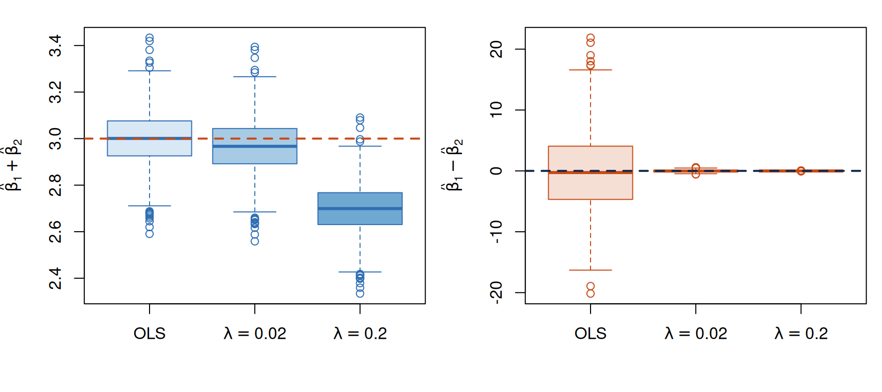
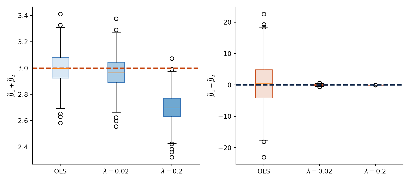
The first two covariates are almost copies. The sum of their coefficients, $\beta_1+\beta_2$ , controls the well-observed combined effect. The difference of their coefficients, $\beta_1-\beta_2$ , controls how that effect is divided between the two covariates. The simulation below compares these two directions directly.

Show the reproducible code

# Re-express the first two coefficients in stable and unstable directions.
beta_sum <- beta_hat[, 1, selected_grid_positions] + beta_hat[, 2, selected_grid_positions]
beta_difference <- beta_hat[, 1, selected_grid_positions] - beta_hat[, 2, selected_grid_positions]
method_labels <- c("OLS", expression(lambda == 0.02), expression(lambda == 0.2))

old_par <- par(no.readonly = TRUE)
par(mfrow = c(1, 2), mar = c(4.5, 4.3, 1.4, 0.8))
boxplot(
  beta_sum,
  names = method_labels,
  ylab = expression(hat(beta)[1] + hat(beta)[2]),
  col = c("#D9E8F5", "#A8CBE5", "#6FA8D1"),
  border = "#2F6FB3"
)
abline(h = 3, lty = 2, lwd = 2, col = "#C84A16")

boxplot(
  beta_difference,
  names = method_labels,
  ylab = expression(hat(beta)[1] - hat(beta)[2]),
  col = c("#F5DFD5", "#EFB89F", "#E28A66"),
  border = "#C84A16"
)
abline(h = 0, lty = 2, lwd = 2, col = "#13294B")

The OLS estimates of beta one plus beta two are concentrated near three, while estimates of beta one minus beta two are widely spread. Ridge greatly reduces the spread in the difference direction, while the stronger penalty shifts the sum downward. — Estimates of the combined and difference directions across 1,000 responses at the same fixed design. Dashed lines mark the true values.

Show the reproducible code

par(old_par)

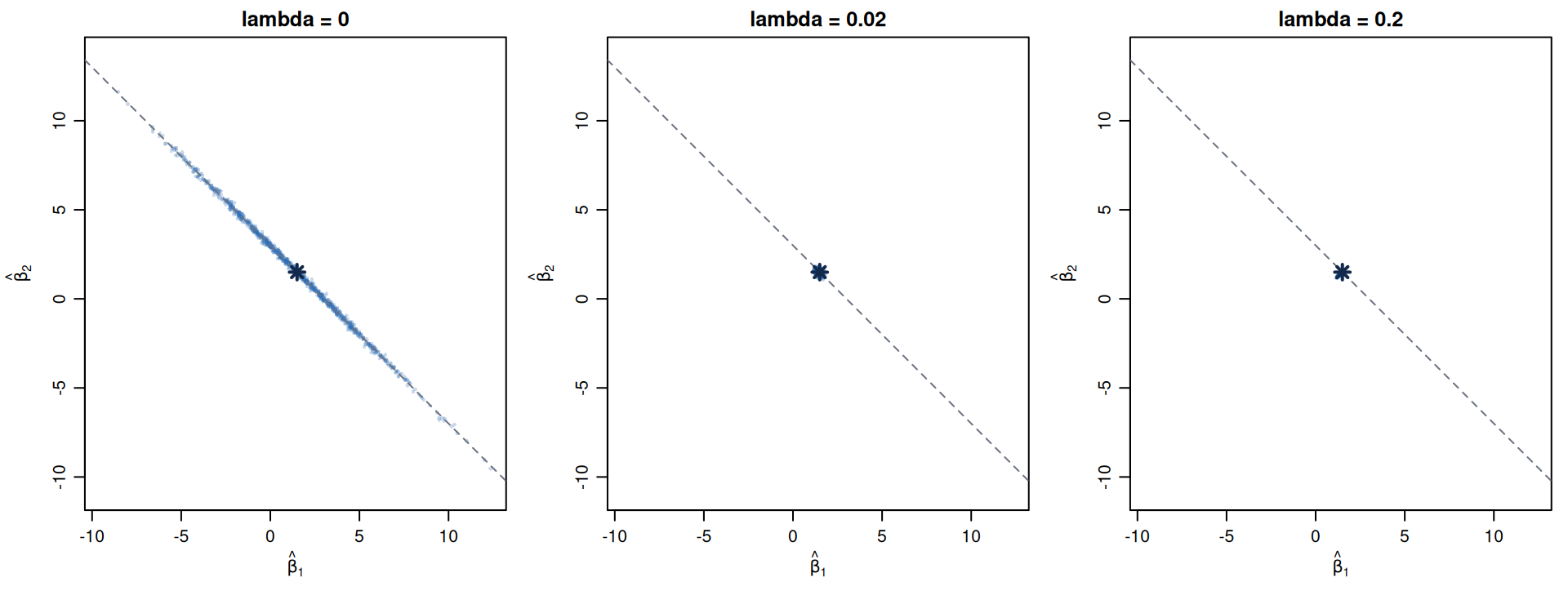
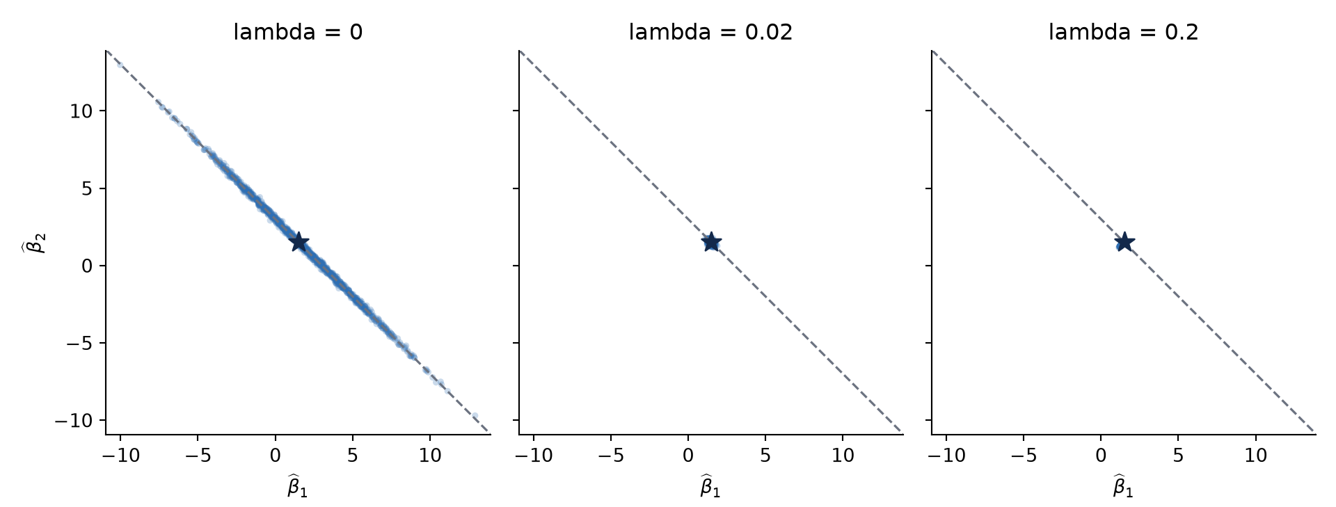
OLS coefficient estimates spread widely along a negatively sloped line. Ridge estimates form progressively tighter clouds as lambda increases, with some movement away from the true point. — Coefficient estimates across 1,000 responses at the same fixed design. The star is the true coefficient pair and the dashed line preserves their true sum.

Show the reproducible code

# Re-express the first two coefficients in stable and unstable directions.
beta_sum = beta_hat[:, 0, selected_grid_positions] + beta_hat[:, 1, selected_grid_positions]
beta_difference = beta_hat[:, 0, selected_grid_positions] - beta_hat[:, 1, selected_grid_positions]
method_labels = ["OLS", r"$\lambda=0.02$", r"$\lambda=0.2$"]

fig, axes = plt.subplots(1, 2, figsize=(9, 4))
sum_box = axes[0].boxplot(
    [beta_sum[:, l] for l in range(3)],
    tick_labels=method_labels,
    patch_artist=True,
)
for patch, color in zip(sum_box["boxes"], ["#D9E8F5", "#A8CBE5", "#6FA8D1"]):
    patch.set_facecolor(color)
    patch.set_edgecolor("#2F6FB3")
axes[0].axhline(3, linestyle="--", linewidth=2, color="#C84A16")
axes[0].set_ylabel(r"$\widehat\beta_1+\widehat\beta_2$")

difference_box = axes[1].boxplot(
    [beta_difference[:, l] for l in range(3)],
    tick_labels=method_labels,
    patch_artist=True,
)
for patch, color in zip(
    difference_box["boxes"], ["#F5DFD5", "#EFB89F", "#E28A66"]
):
    patch.set_facecolor(color)
    patch.set_edgecolor("#C84A16")
axes[1].axhline(0, linestyle="--", linewidth=2, color="#13294B")
axes[1].set_ylabel(r"$\widehat\beta_1-\widehat\beta_2$")

for axis in axes:
    axis.spines[["top", "right"]].set_visible(False)
fig.tight_layout()
plt.show()

OLS estimates the combined direction $\beta_1+\beta_2$ quite precisely, but it estimates the difference direction $\beta_1-\beta_2$ very poorly. The elongated coefficient cloud makes the flat direction visible: moving one coefficient upward and the other downward changes the individual slopes much more than it changes the fitted response.

Ridge sharply reduces variation in the weak difference direction. The stronger penalty also moves the estimated sum below its true value of 3. The figures therefore show the central trade-off directly: less sampling variation in exchange for systematic shrinkage.

Ridge does not reveal which of two redundant covariates is “really” responsible. It prefers a smaller, more balanced coefficient vector among fits that predict similarly. That is useful for stability, but it is not causal identification.

Understand ridge shrinkage mathematically

Derive the ridge solution

The objective introduced earlier is quadratic in $\boldsymbol\beta$ . Differentiate it once and set the gradient to zero:

$\begin{aligned} -\frac{1}{n}\mathbf X^{\mathsf T} (\widetilde{\mathbf y}-\mathbf X\widehat{\boldsymbol\beta}_\lambda) +\lambda\widehat{\boldsymbol\beta}_\lambda &=0,\\ \left(\mathbf X^{\mathsf T}\mathbf X+n\lambda\mathbf I_p\right) \widehat{\boldsymbol\beta}_\lambda &=\mathbf X^{\mathsf T}\widetilde{\mathbf y}. \end{aligned}$

The second line is the ridge normal equation. Relative to OLS, ridge adds $n\lambda\mathbf I_p$ to the slope Gram matrix, increasing each eigenvalue by $n\lambda$ . Therefore,

$\boxed{ \widehat{\boldsymbol\beta}_\lambda = \left(\mathbf X^{\mathsf T}\mathbf X+n\lambda\mathbf I_p\right)^{-1} \mathbf X^{\mathsf T}\widetilde{\mathbf y}. }$

For every $\lambda>0$ , the added diagonal term makes the matrix invertible and the solution unique. At $\lambda=0$ , the formula also requires $\mathbf X$ to have full column rank.

The inverse is useful notation, but numerical code should solve the displayed linear system rather than explicitly construct an inverse. The simulation already used a linear-system solve for every penalty. The following calculation takes the fitted coefficient vector at $\lambda=0.2$ from its final repetition and verifies that it satisfies the normal equation.

Show the reproducible code

# Check the stored ridge solution from the final repetition.
lambda <- 0.2
l <- match(lambda, lambda_grid_r)
normal_equation_residual <-
  (gram + n * lambda * diag(p)) %*%
    beta_hat[repetitions, , l] -
  crossprod(X, y_centered)

knitr::kable(
  data.frame(
    feature = feature_names,
    true_slope = beta,
    ridge_estimate = beta_hat[repetitions, , l]
  ),
  digits = c(0, 2, 4),
  row.names = FALSE,
  caption = "A direct ridge solve at lambda = 0.2"
)

A direct ridge solve at lambda = 0.2
feature	true_slope	ridge_estimate
x1	1.50	1.5072
x2	1.50	1.5393
x3	1.00	0.7920
x4	0.75	0.6579
x5	0.50	0.4628
x6	0.00	-0.0559

Show the reproducible code

cat(
  "\nMaximum absolute normal-equation residual:",
  format(max(abs(normal_equation_residual)), scientific = TRUE)
)


Maximum absolute normal-equation residual: 5.684342e-14

Show the reproducible code

# Check the stored ridge solution from the final repetition.
lam = 0.2
l = int(np.flatnonzero(np.isclose(lambda_grid_py, lam))[0])
normal_equation_residual = (
    (gram + n * lam * np.eye(p)) @ beta_hat[repetitions - 1, :, l]
    - X.T @ y_centered
)

from IPython.display import HTML, display

ridge_table_py = pd.DataFrame(
    {
        "feature": feature_names,
        "true_slope": beta,
        "ridge_estimate": beta_hat[repetitions - 1, :, l],
    }
)
print("A direct ridge solve at lambda = 0.2")

A direct ridge solve at lambda = 0.2

Show the reproducible code

display(HTML(ridge_table_py.to_html(
    index=False,
    formatters={
        "true_slope": "{:.2f}".format,
        "ridge_estimate": "{:.4f}".format,
    },
)))

<IPython.core.display.HTML object>

Show the reproducible code

print(
    "Maximum absolute normal-equation residual:",
    f"{np.max(np.abs(normal_equation_residual)):.3e}",
)

Maximum absolute normal-equation residual: 2.842e-14

The near-zero residual is a numerical check of the normal equation. The table also illustrates a substantive point: the estimates need not be individually close to their true coefficients for every realized response. Ridge improves stability and can improve average prediction; it does not guarantee exact recovery from one noisy sample.

What happens at the two ends of the path?

If $\mathbf X$ has full column rank, then

$\lim_{\lambda\downarrow0} \widehat{\boldsymbol\beta}_\lambda = \widehat{\boldsymbol\beta}_{\mathrm{OLS}}.$

If the design is rank deficient, OLS has multiple coefficient solutions. In that case, the ridge path approaches the Moore-Penrose minimum-norm least-squares solution as $\lambda\downarrow0$ .

At the other end,

$\lim_{\lambda\to\infty} \widehat{\boldsymbol\beta}_\lambda =\mathbf 0.$

The fitted centered response approaches zero as the slopes vanish. Adding the response mean back gives the constant $\bar y$ on the original response scale.

Orthogonal design: shrink every slope by the same fraction

The easiest case makes shrinkage completely transparent. Suppose the standardized covariates are orthogonal, so

$\mathbf X^{\mathsf T}\mathbf X=n\mathbf I_p.$

Substituting this identity into the ridge solution gives

$\begin{aligned} \widehat{\boldsymbol\beta}_\lambda &=(n\mathbf I_p+n\lambda\mathbf I_p)^{-1} \mathbf X^{\mathsf T}\widetilde{\mathbf y}\\ &=\frac{1}{1+\lambda} \left(\mathbf X^{\mathsf T}\mathbf X\right)^{-1} \mathbf X^{\mathsf T}\widetilde{\mathbf y}\\ &=\boxed{ \frac{1}{1+\lambda} \widehat{\boldsymbol\beta}_{\mathrm{OLS}} }. \end{aligned}$

Every OLS slope is multiplied by the same number between zero and one. For example, $\lambda=0.25$ retains $1/1.25=0.8$ of every OLS coefficient; $\lambda=1$ retains one half.

In this orthogonal setting, ridge does not create exact zeros. For finite $\lambda$ , the multiplier $1/(1+\lambda)$ is positive. A nonzero OLS slope becomes smaller but remains nonzero.

General designs: shrink principal directions

Real covariates are not usually orthogonal. The singular value decomposition provides the right coordinate system. Let the rank- $r$ thin SVD be

$\mathbf X=\mathbf U_r\mathbf D_r\mathbf V_r^{\mathsf T},$

where $\mathbf U_r\in\mathbb R^{n\times r}$ , $\mathbf D_r\in\mathbb R^{r\times r}$ , $\mathbf V_r\in\mathbb R^{p\times r}$ , and

$\mathbf D_r=\operatorname{diag}(d_1,\ldots,d_r), \qquad d_1\ge\cdots\ge d_r>0.$

The values $d_j$ are singular values. Their squares are the positive eigenvalues of $\mathbf X^{\mathsf T}\mathbf X$ . The columns $\mathbf v_j$ of $\mathbf V_r$ are coefficient-space directions, and $\mathbf X\mathbf v_j=d_j\mathbf u_j$ tells us how visible each direction is in the observed design.

Substitute the SVD into the ridge solution:

$\begin{aligned} \widehat{\boldsymbol\beta}_\lambda &= \mathbf V_r(\mathbf D_r^2+n\lambda\mathbf I_r)^{-1} \mathbf D_r\mathbf U_r^{\mathsf T}\widetilde{\mathbf y}\\ &= \sum_{j=1}^r \mathbf v_j \frac{d_j}{d_j^2+n\lambda} \mathbf u_j^{\mathsf T}\widetilde{\mathbf y}. \end{aligned}$

If $r<p$ , coefficient directions in the null space of $\mathbf X$ do not change the fitted response. Ridge sets those components to zero because any nonzero null-space component would increase the penalty without improving fit. This is how the penalty selects one unique coefficient vector when the design is rank deficient.

For $\lambda=0$ , the coefficient along $\mathbf v_j$ divides by $d_j$ . If $d_j$ is tiny, even a small noise component $\mathbf u_j^{\mathsf T}\boldsymbol\epsilon$ is magnified by $1/d_j$ . This is the algebraic source of unstable OLS coefficients.

Within each observed direction, ridge multiplies the corresponding minimum-norm OLS coefficient by

$\boxed{ \rho_j(\lambda) = \frac{d_j^2}{d_j^2+n\lambda}. }$

When $d_j^2$ is large relative to $n\lambda$ , $\rho_j(\lambda)$ is near one and ridge largely preserves that direction. A small singular value marks a weakly identified direction, so the same penalty shrinks it much more strongly.

This factor gives the direction-wise bias-variance trade-off. Under $\boldsymbol\mu=\mathbf X\boldsymbol\beta$ ,

$E\!\left( \mathbf v_j^{\mathsf T}\widehat{\boldsymbol\beta}_\lambda \mid\mathbf X \right) = \rho_j(\lambda)\, \mathbf v_j^{\mathsf T}\boldsymbol\beta,$

and

$\operatorname{Var}\!\left( \mathbf v_j^{\mathsf T}\widehat{\boldsymbol\beta}_\lambda \mid\mathbf X \right) = \frac{\sigma^2d_j^2} {(d_j^2+n\lambda)^2}.$

When $\lambda=0$ , the variance is $\sigma^2/d_j^2$ , which is large when the design contains little information in direction $\mathbf v_j$ . A positive penalty reduces this variance, but it also moves the expected coefficient toward zero.

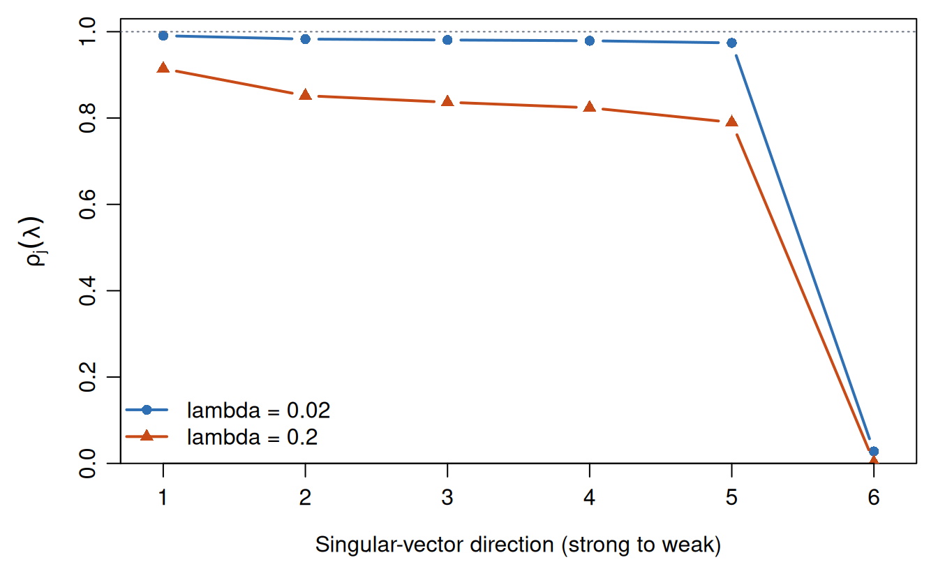
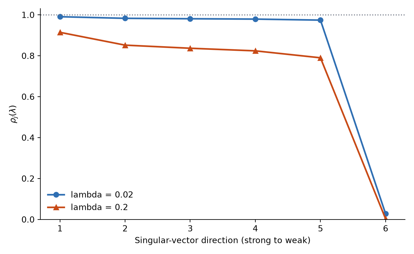
Shrinkage factors are near one for the strongest directions and much smaller for the weakest direction, especially under the larger penalty. — Ridge shrinkage factors along the six singular-vector directions of the fixed design. Directions are ordered from strongest to weakest.

The weakest direction in this design is approximately the difference between the first two covariates. The true signal mainly uses their stable sum. Ridge therefore removes a large amount of noise amplification in a direction that contributes little to the true fitted mean. This alignment is why a modest penalty can help substantially here.

The fitted centered response has an especially simple form:

$\begin{aligned} \mathbf X\widehat{\boldsymbol\beta}_\lambda &= \mathbf U_r \operatorname{diag}\{\rho_1(\lambda),\ldots,\rho_r(\lambda)\} \mathbf U_r^{\mathsf T}\widetilde{\mathbf y}. \end{aligned}$

Ridge keeps every observed singular direction but attenuates it continuously. Unlike lasso, ordinary ridge does not usually set individual slopes exactly to zero.

Connect stability to prediction

Return to the original measurement units

We have seen how ridge stabilizes slopes in a centered, standardized problem. For data recorded in their original units, how do we obtain that setting and translate the fitted model back?

Let $\mathbf X_{\mathrm{raw}}\in\mathbb R^{n\times p}$ contain the raw covariates. For each nonconstant covariate $j$ , calculate its training-sample mean and scale:

$\bar x_j=\frac{1}{n}\sum_{i=1}^n x_{\mathrm{raw},ij}, \qquad s_j= \left\{ \frac{1}{n}\sum_{i=1}^n(x_{\mathrm{raw},ij}-\bar x_j)^2 \right\}^{1/2}.$

The centered, standardized covariate matrix has entries

$X_{ij}=\frac{x_{\mathrm{raw},ij}-\bar x_j}{s_j}.$

Thus every column of $\mathbf X$ has mean zero and average squared value one. We center the response without dividing by its standard deviation:

$\bar y=\frac{1}{n}\sum_{i=1}^n y_i, \qquad \widetilde{\mathbf y}=\mathbf y-\bar y\mathbf 1_n.$

These are the transformations used in the simulation code. The numerical size of a raw slope depends on its measurement unit. Converting a covariate from meters to millimeters divides its slope by 1,000 even though the scientific relationship is unchanged. Standardization prevents this arbitrary unit choice from determining how strongly a covariate is penalized.

Leave the intercept unpenalized

Centering separates the baseline level from the slopes. Ridge fits $\bar y$ without penalty and applies shrinkage only to the $p$ slopes. If every response increases by 100, every fitted value should also increase by 100. The penalty should not resist that translation.

For a raw covariate vector $\mathbf x_{\mathrm{raw}}\in\mathbb R^p$ , the fitted value is

$\widehat y(\mathbf x_{\mathrm{raw}}) = \bar y+ \sum_{j=1}^p \widehat\beta_j \frac{x_{\mathrm{raw},j}-\bar x_j}{s_j},$

where $\widehat\beta_j$ is the fitted slope on the standardized scale at the chosen penalty. Expanding this expression gives slopes and an intercept in the original units:

$\boxed{ \widehat\beta_{\mathrm{raw},j}=\frac{\widehat\beta_j}{s_j}, \qquad \widehat\beta_{\mathrm{raw},0} =\bar y-\sum_{j=1}^p\bar x_j\widehat\beta_{\mathrm{raw},j}. }$

Divide each fitted slope by its covariate’s scale, then adjust the intercept for the covariate means. The predictions are unchanged:

$\widehat y(\mathbf x_{\mathrm{raw}}) =\widehat\beta_{\mathrm{raw},0} +\sum_{j=1}^p x_{\mathrm{raw},j}\widehat\beta_{\mathrm{raw},j}.$

Preprocessing is part of the fitted model

The denominator $n$ in $s_j$ is a convention. Using $n-1$ changes the numerical meaning of $\lambda$ . During cross-validation, all means and scales must be learned inside each training fold. The tuning lecture implements that procedure.

Does greater stability improve prediction?

Smaller slope variance is encouraging, but it is not the final goal. A very large penalty would make the slope estimates almost perfectly stable by making them almost zero; that could badly underfit the true mean. For each repetition, we record the observed training MSE and the observed MSE on its independent test response. We then average those values over the 1,000 repetitions and compare them with their theoretical expectations.

For a fixed $\lambda$ , define the ridge smoother matrix, including the unpenalized intercept, as

$\mathbf H_\lambda = \frac{1}{n}\mathbf 1_n\mathbf 1_n^{\mathsf T} + \mathbf X \left(\mathbf X^{\mathsf T}\mathbf X+n\lambda\mathbf I_p\right)^{-1} \mathbf X^{\mathsf T}.$

Then $\widehat{\mathbf y}_\lambda=\mathbf H_\lambda\mathbf y$ . All expectations in this section condition on the fixed matrix $\mathbf X$ . You do not need to derive the following formulas. Focus on identifying the squared-bias, estimation-variance, and independent-response noise terms and on using them to interpret the risk curves. The training and test risks are

$\begin{aligned} E\{\operatorname{MSE}_{\mathrm{train}}(\lambda)\mid\mathbf X\} &= \frac{1}{n} \lVert(\mathbf I_n-\mathbf H_\lambda)\boldsymbol\mu\rVert_2^2 + \frac{\sigma^2}{n} \operatorname{tr}\!\left\{ (\mathbf I_n-\mathbf H_\lambda)^{\mathsf T} (\mathbf I_n-\mathbf H_\lambda) \right\},\\ E\{\operatorname{MSE}_{\mathrm{test}}(\lambda)\mid\mathbf X\} &= \frac{1}{n} \lVert(\mathbf I_n-\mathbf H_\lambda)\boldsymbol\mu\rVert_2^2 + \frac{\sigma^2}{n} \operatorname{tr}(\mathbf H_\lambda^{\mathsf T}\mathbf H_\lambda) + \sigma^2. \end{aligned}$

The first term in the test expression is the mean squared bias of the fitted mean vector, the second is estimation variance, and the final $\sigma^2$ is the noise in the independent test response. The formulas explain what the simulation should approach after many repetitions. One realized training or test MSE can still differ from its expectation.

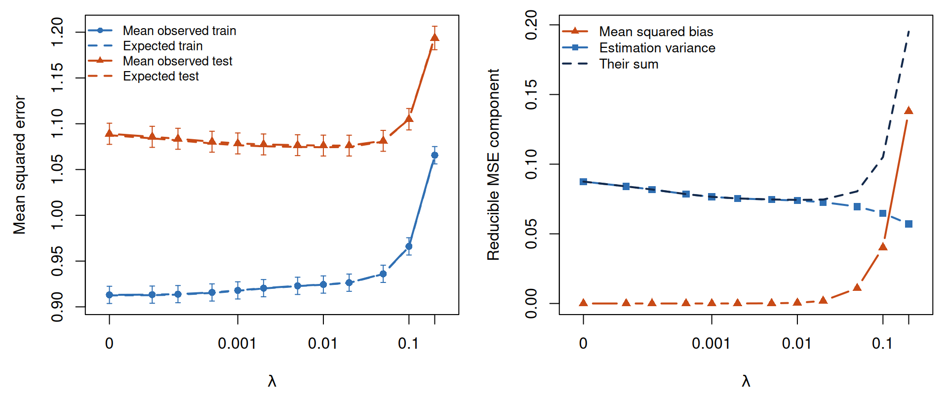
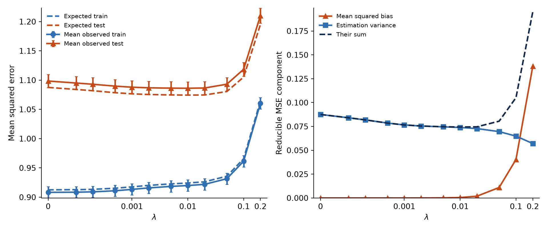
Mean training error rises with stronger penalization. Mean independent-test error first decreases and later increases. The mean-squared-bias component rises while the estimation-variance component falls. — Risk over the practically relevant part of the penalty path, from OLS through lambda = 0.2. Left: mean observed training and independent-test MSE, together with their theoretical expectations. Right: mean squared bias and estimation variance of the fitted mean.

Mean training error rises as the penalty strengthens because ridge places more weight on keeping slopes small relative to minimizing training RSS. That rise is not evidence that the method is failing. It is the visible cost of restricting how closely the model follows an observed response.

Mean independent-test error initially falls. In that region, the variance reduction is worth more than the added squared bias. Eventually the penalty becomes too strong, genuine mean structure is erased, and squared bias dominates. The useful $\lambda$ lies between the unstable OLS endpoint and the nearly constant-model endpoint.

For this design, expected test MSE falls from $1.0875$ at $\lambda=0$ to $1.0746$ at $\lambda=0.02$ . At the same time, the quadratic loss condition number falls from about $3748.5$ to $104.9$ . Increasing the penalty to $0.2$ improves the condition number further, to about $11.7$ , but expected test MSE rises to $1.1951$ because squared bias has become too large. Numerical stability and predictive accuracy are related, but they are not the same target.

Bias and variance in plain language. Across repeated response samples, bias is the systematic shift in the average fitted mean caused by shrinkage. Variance is how much the fitted mean changes from one response sample to another. Ridge helps when the decrease in variance is larger than the increase in squared bias. One observed test MSE is noisy; the curve summarizes average behavior over repetitions.

A U-shape is a result, not a law

The simulation was designed so the true signal has little contribution in its weakest direction, making ridge especially helpful. If important signal lay mostly in a weak singular direction, shrinkage bias would grow sooner. If the design were already well conditioned and $n$ were large, OLS variance might be small enough that ridge offers little improvement.

Connecting back to Week 2

Week 2 used a matrix that maps the response vector to fitted values. Ridge has the same linear-smoother structure. The matrix $\mathbf H_\lambda$ defined in the prediction-risk section includes the fitted response mean in its first term and the shrunken slope contribution in its second. For a fixed $\lambda$ , the fitted vector is

$\widehat{\mathbf y}_\lambda=\mathbf H_\lambda\mathbf y.$

For $\lambda>0$ , $\mathbf H_\lambda$ is not a projection matrix. Ridge still estimates all $p$ slopes, but each principal direction responds by only the fraction $\rho_j(\lambda)$ . This leads to a fractional measure of complexity rather than a count of nonzero coefficients.

Effective degrees of freedom

Week 2 connected model complexity to how strongly fitted values respond to the observed responses. For a linear smoother, that effective complexity is the trace of its smoother matrix. Ridge therefore has

$\begin{aligned} \operatorname{df}_{\mathrm{eff}}(\lambda) &=\operatorname{tr}(\mathbf H_\lambda)\\ &=\boxed{1+\sum_{j=1}^r\rho_j(\lambda)}. \end{aligned}$

The leading one is the unpenalized intercept. At $\lambda=0$ and full column rank, the total is $p+1$ . As $\lambda$ grows, every $\rho_j(\lambda)$ decreases and the total approaches one. Ridge can therefore have all slopes nonzero while using less than $p+1$ effective degrees of freedom.

Week 2 showed that training error is optimistic because the same responses are used to fit and evaluate a model. Under the fixed- $\mathbf X$ noise model used above, and for a fixed $\lambda$ , ridge has the expected gap

$E\{\operatorname{MSE}_{\mathrm{test}}(\lambda)\mid\mathbf X\} - E\{\operatorname{MSE}_{\mathrm{train}}(\lambda)\mid\mathbf X\} = \frac{2\sigma^2}{n}\operatorname{tr}(\mathbf H_\lambda).$

This equation compares expectations over repeated observed and independent test responses. A single observed test MSE can be above or below its own expectation. As $\lambda$ grows, ridge responds less to training noise, so its effective degrees of freedom and its average optimism both decrease.

A software column named Df may mean something else

Some regularization packages use Df to count nonzero slopes. That count usually remains $p$ for ridge. It is not the fractional effective degrees of freedom $\operatorname{tr}(\mathbf H_\lambda)$ .

Limitations

Ridge is powerful, but its scope is specific.

It does not repair a wrong mean structure. If the response depends nonlinearly on the covariates and the required features are absent, shrinking a linear fit does not create them.
It does not automatically select variables. Ridge coefficients are usually small but nonzero. If a sparse variable list is required, a different penalty or a separate decision rule is needed.
It does not identify individual causal effects. It stabilizes a preferred combination, often by sharing weight among correlated covariates. That is different from establishing which variable is causal.
It depends on preprocessing and the penalty convention. A numerical value called “lambda” is not directly comparable across software until the loss normalization and standardization rules are aligned.
It does not choose its own tuning parameter. Training RSS prefers $\lambda=0$ . Selecting $\lambda$ requires an estimate of future prediction performance, such as cross-validation or generalized cross-validation.

The next lecture addresses the computational side: gradient descent, package conventions, cross-validation without preprocessing leakage, the minimum-error and one-standard-error rules, and one final test-set evaluation.

Review

Check your understanding

Two covariates are almost identical. Why can their OLS slopes vary greatly even when the fitted response changes little?
Why do we center the response and leave the intercept outside the ridge penalty?
Why does ridge shrink a singular-vector direction with a small $d_j$ more strongly?
Can ridge produce lower prediction MSE even though its coefficient estimator is biased? Explain what must compensate for the squared bias.

Key ideas

Near redundancy creates a flat loss direction and high OLS coefficient variance.
Ridge adds a quadratic penalty, stabilizing the same directions that are statistically weak.
Standardization gives the penalty a comparable meaning across covariates; the intercept remains unpenalized.
Ridge shrinks singular direction $j$ by $\rho_j(\lambda)=d_j^2/(d_j^2+n\lambda)$ .
Positive $\lambda$ trades added squared bias for lower variance. The penalty must be tuned against a prediction target, not training RSS.

Next: optimize ridge, align R and Python penalty conventions, and tune $\lambda$ with cross-validation.

References and further reading

Hoerl and Kennard (1970) introduced ridge estimation for nonorthogonal regression problems and emphasized that a biased estimator can achieve smaller mean squared error.
James, Witten, Hastie, Tibshirani, and Taylor, An Introduction to Statistical Learning, Chapter 6, give an accessible treatment of shrinkage methods. Hastie, Tibshirani, and Friedman, The Elements of Statistical Learning, Chapter 3, provide a more advanced account of linear shrinkage and principal-component directions.

Footnotes

We use $n^{-1}\sum_{i=1}^n X_{ij}^2=1$ for each already centered column. This convention fixes the numerical scale of $\lambda$ .↩︎