Skip to main content

The Curse of Dimensionality

Nearest neighbors in many dimensions

On this page

• Example: Handwritten Digit Data
• The Curse of Dimensionality
• An Experiment
• Discussion

← Week 5 overview · K-Nearest Neighbors

Example: Handwritten Digit Data

Let’s consider another example using handwritten digits. Each observation is a $16\times16$ pixel image, so there are $p=256$ variables. Each variable records the grayscale value at one pixel. Can nearest neighbors recognize the digit from these pixel values?

R

  # Handwritten Digit Recognition Data
  library(ElemStatLearn)

  # the first column is the true digit
  dim(zip.train)

[1] 7291  257

  dim(zip.test)

[1] 2007  257

  # look at one sample
  image(zip2image(zip.train, 1), col=gray(256:0/256), zlim=c(0,1),
        xlab="", ylab="", axes = FALSE)

[1] "digit  6  taken"

Python

Use the original training data and test data. The files contain the same observations and split as the R data. Save them in data/knn and run the code from the folder containing data.

import numpy as np
import matplotlib.pyplot as plt
from pathlib import Path

# Handwritten digit recognition data; the first column is the true digit.
zip_train = np.loadtxt(Path("data/knn/zip-train.csv.gz"), delimiter=",")
zip_test = np.loadtxt(Path("data/knn/zip-test.csv.gz"), delimiter=",")
print(zip_train.shape)

(7291, 257)

print(zip_test.shape)

(2007, 257)

# Look at the same sample as in R.
print("digit", int(zip_train[0, 0]), "taken")

digit 6 taken

plt.figure(figsize=(6, 6))
plt.imshow(zip_train[0, 1:].reshape(16, 16), cmap="gray_r",
           vmin=0, vmax=1, interpolation="nearest")
plt.axis("off")
plt.show()

The training data contain 7,291 images, and the test data contain 2,007 images. We use 3NN to predict the digits in the test data and examine the error rate and confusion matrix. The matrix has predicted digits in rows and observed digits in columns.

R

  library(class)
  # fit 3nn model and calculate the error
  knn.fit <- knn(zip.train[, 2:257], zip.test[, 2:257], zip.train[, 1], k=3)

  # overall prediction error
  mean(knn.fit != zip.test[,1])

[1] 0.05580468

  # the confusion matrix
  table(knn.fit, zip.test[,1])

       
knn.fit   0   1   2   3   4   5   6   7   8   9
      0 355   0   7   2   0   2   3   0   4   1
      1   0 257   0   0   2   0   1   1   0   0
      2   2   0 182   2   0   2   1   1   1   0
      3   0   0   1 153   0   6   0   1   3   0
      4   0   3   2   0 182   0   2   4   0   3
      5   0   0   0   7   2 144   0   0   1   0
      6   0   2   0   0   2   1 163   0   0   0
      7   1   2   2   1   3   0   0 138   1   4
      8   0   0   4   0   1   1   0   1 153   1
      9   1   0   0   1   8   4   0   1   3 168

Python

import pandas as pd
from sklearn.neighbors import KNeighborsClassifier

# Fit 3NN and calculate the test error.
knn_fit = KNeighborsClassifier(n_neighbors=3, weights="uniform")
knn_fit.fit(zip_train[:, 1:257], zip_train[:, 0])
test_pred = knn_fit.predict(zip_test[:, 1:257])
print(np.mean(test_pred != zip_test[:, 0]))

0.05530642750373692

# Rows are predictions; columns are observed digits.
print(pd.crosstab(pd.Series(test_pred.astype(int), name="Prediction"),
                  pd.Series(zip_test[:, 0].astype(int), name="Observed")))

Observed      0    1    2    3    4    5    6    7    8    9
Prediction                                                  
0           355    0    8    3    0    5    3    0    4    2
1             0  258    0    0    2    0    1    1    0    0
2             3    0  183    2    0    3    1    1    3    0
3             0    0    1  153    0    3    0    1    4    0
4             0    3    1    0  183    0    2    4    0    3
5             0    0    0    6    2  144    0    0    1    0
6             0    2    0    0    2    0  163    0    0    0
7             0    1    2    1    2    0    0  138    1    4
8             0    0    3    0    1    1    0    1  151    0
9             1    0    0    1    8    4    0    1    2  168

Most predictions lie on the diagonal of the confusion matrix, so 3NN recognizes most test digits correctly. There are 256 predictors here. Does this mean that nearest neighbors will work well whenever there are many predictors?¹

The Curse of Dimensionality

Many practical problems have high-dimensional data. The handwritten digits have $16\times16=256$ pixel measurements, and genetic studies can contain many thousands of gene-expression measurements. For a fixed sample size $n$, observations become sparse as the number of variables $p$ increases. A target point may then have few training observations close to it, making local averaging less effective.

To see why, consider $n=1000$ observations drawn uniformly from a $p$-dimensional unit cube. We want to use $k=10$ neighbors. If the regression function changes little over a small neighborhood, averaging responses from that neighborhood can have small bias.

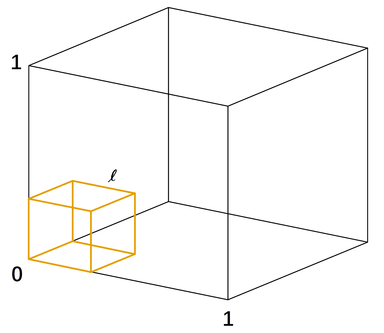
For $p=2$, a square with side length $\ell=0.1$ has area $0.1^2$. It contains $1000\times0.1^2=10$ observations in expectation. More generally, a cube of side length $\ell$ contained in the unit cube has expected count $n\ell^p$. To obtain an expected count of $k$, we need

$$\ell^p=\frac{k}{n}.$$

Keeping $k/n=10/1000$ fixed gives:

• If $p=2$, $\ell=0.1$.
• If $p=10$, $\ell\approx0.63$.
• If $p=100$, $\ell\approx0.955$.

As dimension increases, the cube must span much more of each coordinate’s range to contain the same expected number of observations. The side length $\ell$ describes this cube; it is not the distance of every neighbor from the target in every coordinate. The calculation shows why a neighborhood can stop being local. If the regression function changes substantially over that neighborhood, the bias can be large. Decreasing $k$ may not solve the problem because even the closest observations can be far away, while averaging fewer noisy responses increases variance.

A small cube of side length ell inside a unit cube.

An Experiment

Let’s examine this issue with a small simulation. Generate $p=10$ independent covariates, each uniformly distributed on $(0,1)$, and let the outcome depend on the first three predictors:

$$y_i=X_{i1}+X_{i2}+X_{i3}+\epsilon_i, \qquad \epsilon_i\sim N(0,0.5^2),$$

with errors independent of the covariates and one another. Thus $f(\mathbf x)=x_1+x_2+x_3$. At the target $\mathbf x_0=(0,0,\ldots,0)^\mathsf T$, the true mean is $f(\mathbf x_0)=0$. This target is a corner of the covariate support.

Recall the repeated simulations from ridge regression. Here, we generate a new training dataset, fit 5NN, and predict at the same target in each repetition. Repeating this 300 times estimates

$$E\left[\left\{\widehat f(\mathbf x_0)-f(\mathbf x_0)\right\}^2\right].$$

This is mean squared error for estimating the regression function at the target. We compare the prediction with the true mean, so this quantity does not include a new noisy outcome at $\mathbf x_0$. The expectation averages over the randomly generated training covariates and responses.

R

  # Let's try a new package FNN
  library(FNN)
  p = 10
  n = 100

  # the target prediction point
  # be careful that this needs to be a 1xp matrix
  x0 = matrix(rep(0, p), nrow = 1, ncol = p)

  # number of simulations
  nsim = 300

  # vector to store predicted values
  allerror = rep(NA, nsim)

  for (l in 1:nsim)
  {
    # generate data
    X = matrix(runif(n*p), nrow = n, ncol = p)
    y = X[, 1] + X[, 2] + X[, 3] + rnorm(n, sd = 0.5)

    # "5-nearest neighbor" regression using the FNN package
    # for this question, use the "brute force" algorithm to search for the NNs
    knn.fit = knn.reg(train = X, test = x0, y = y,
                      k = 5, algorithm = "brute")

    # record the prediction error of this run
    # the truth f(x_0) is 0
    allerror[l] = (knn.fit$pred - 0)^2
  }

  # the prediction error
  mean(allerror)

[1] 0.9483551

Python

from sklearn.neighbors import KNeighborsRegressor

p = 10
n = 100

# The target must have one row and p columns.
x0 = np.zeros((1, p))

# Number of simulations and storage for the squared errors.
nsim = 300
allerror = np.full(nsim, np.nan)

for l in range(nsim):
    X = np.random.uniform(0, 1, size=(n, p))
    y = X[:, 0] + X[:, 1] + X[:, 2] + np.random.normal(0, 0.5, n)

    # Use brute-force neighbor search, as in the R example.
    knn_fit = KNeighborsRegressor(n_neighbors=5, weights="uniform",
                                  algorithm="brute")
    knn_fit.fit(X, y)
    allerror[l] = (knn_fit.predict(x0)[0] - 0)**2

print(np.mean(allerror))

1.0438422123340028

Each entry of allerror is a squared error from one newly generated dataset; its average estimates the displayed expectation. At this corner, nearby training observations still have positive values in the first three coordinates, so their mean responses can be well above the target’s true mean of zero. The numerical average varies across runs.

Practice question

Use the same code to calculate the mean squared error at $\mathbf x_0=(1,1,1,0,\ldots,0)^\mathsf T$, another corner of the support. Here $f(\mathbf x_0)=3$. What are the errors when $p=5,10$, and $20$? The example below sets $p=20$; change $p$ to examine the other dimensions.

R

  # Let's try a new package FNN
  library(FNN)
  p = 20
  n = 100

  # the target prediction point
  # be careful that this needs to be a 1xp matrix
  x0 = matrix(c(rep(1, 3), rep(0, p-3)), nrow = 1, ncol = p)

  # number of simulations
  nsim = 300

  # vector to store predicted values
  allerror = rep(NA, nsim)

  for (l in 1:nsim)
  {
    # generate data
    X = matrix(runif(n*p), nrow = n, ncol = p)
    y = X[, 1] + X[, 2] + X[, 3] + rnorm(n, sd = 0.5)

    # "5-nearest neighbor" regression using the FNN package
    # for this question, use the "brute force" algorithm to search for the NNs
    knn.fit = knn.reg(train = X, test = x0, y = y,
                      k = 5, algorithm = "brute")

    # record the prediction error of this run
    # the truth f(x0) is 3
    allerror[l] = (knn.fit$pred - 3)^2
  }

  # the prediction error
  mean(allerror)

Python

from sklearn.neighbors import KNeighborsRegressor

p = 20
n = 100

# The first three target coordinates are one; the others are zero.
x0 = np.array([[1, 1, 1] + [0] * (p - 3)])

nsim = 300
allerror = np.full(nsim, np.nan)

for l in range(nsim):
    X = np.random.uniform(0, 1, size=(n, p))
    y = X[:, 0] + X[:, 1] + X[:, 2] + np.random.normal(0, 0.5, n)

    knn_fit = KNeighborsRegressor(n_neighbors=5, weights="uniform",
                                  algorithm="brute")
    knn_fit.fit(X, y)
    allerror[l] = (knn_fit.predict(x0)[0] - 3)**2

print(np.mean(allerror))

Discussion

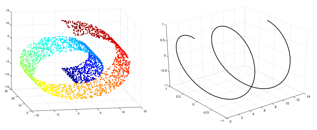
Why, then, did 3NN perform well in the handwritten digit example? The pixel values may have an approximately lower-dimensional structure: they do not vary as 256 unrelated measurements. Distances in the full pixel space can still identify similar digits, and the digit classes may be well separated along that structure. The test performance is consistent with this explanation; it does not prove that an equivalent lower-dimensional representation exists.

Dimension reduction is an important topic in statistical learning and machine learning. Methods such as sliced inverse regression (Li, 1991) and UMAP (McInnes et al., 2018) investigate lower-dimensional representations of data.

A rolled surface and a curved line illustrate lower-dimensional structure in three-dimensional space.

Image from Cayton (2005).

Return to the simulation above. What if all covariates were highly linearly dependent? Would that give an approximately lower-dimensional representation and potentially improve prediction accuracy? Can you use a simulation study to investigate this?

Footnotes

1. The R and Python functions can resolve tied class votes differently, so their test errors need not be exactly equal.