Skip to main content

Classification: Probabilities, Decisions, and Learning Error

On this page

• Learning goals
• From a probability to a class decision
• The Bayes classifier
• Losses for probability predictions
• Bias and variance of an estimated probability
• A KNN experiment
• How probability error becomes classification error
• Unequal error costs
• Check your understanding
• Key ideas
• References and further reading

← Week 6 overview · Previous: K-Nearest Neighbors · Next: Evaluating Classification Models

In the KNN lecture, we averaged nearby binary labels to estimate a class probability. We then compared that probability with a cutoff to predict a class. These two steps lead to two different questions: How accurately have we estimated the probability, and how often will the resulting class decision be wrong?

Learning goals

By the end of this lecture, you should be able to:

• distinguish a class probability, an estimated probability, and a class decision;
• derive the Bayes classifier and explain why it can still make errors;
• explain what squared loss and log loss measure for probability predictions;
• connect probability bias and variance to classification error; and
• explain how unequal error costs change the decision cutoff.

From a probability to a class decision

We start with one predictor $x$ and a binary response $Y\in\{0,1\}$. Write

$$p(x)=P(Y=1\mid X=x)=E(Y\mid X=x).$$

Because $Y$ is either zero or one, its conditional mean is the probability of class 1. A fitted method estimates this probability by $\widehat p(x)$. For example, KNN estimates it by the fraction of class-1 observations among the nearest neighbors.

For a cutoff $t$, the fitted class decision is

$$\widehat d(x)=I\{\widehat p(x)\geq t\}.$$

Here $I\{\cdot\}$ equals one when the condition holds and zero otherwise. We use $t=1/2$ initially. Whenever we change the cutoff, we will state its value. The same notation works with several predictors by letting $x$ represent their observed values.

Two examples show why probability estimation and classification need separate treatment:

• Estimates of $0.60$ and $0.95$ give the same class decision, although they express very different probabilities.
• Estimates of $0.49$ and $0.51$ are close, but give different class decisions.

Guiding question. How does error in an estimated probability become error in a class decision?

The Bayes classifier

First suppose that we know the true probability $p(x)$. At a fixed predictor value, there are only two possible decisions:

Decision	When is it wrong?	Probability of an error
Predict class 0	$Y=1$	$p(x)$
Predict class 1	$Y=0$	$1-p(x)$

We should predict class 1 when $1-p(x)\leq p(x)$. Thus the Bayes classifier under equal error costs is

$$\boxed{d^*(x)=I\{p(x)\geq 1/2\}.}$$

At $p(x)=1/2$, either decision has the same error probability. Knowing the true probability does not mean knowing the next outcome. If $p(x)=0.7$, the Bayes rule predicts class 1 and is still wrong 30 percent of the time at that $x$.

Classification error as expected loss

For a decision rule $d$, the $0$-$1$ loss records whether its decision is wrong:

$$L\{d(x),y\}=I\{d(x)\neq y\}.$$

The risk is the expected loss on a new observation. Under $0$-$1$ loss, it is the population classification error:

$$R(d)=E\left[I\{d(X)\neq Y\}\right]=P\{d(X)\neq Y\}.$$

The expectation averages over new predictor values and their outcomes. One test sample estimates this risk; it does not reveal its exact value.

The Bayes rule chooses the smaller conditional error at every $x$, so its risk is

$$\boxed{R^*=R(d^*)=E\left[\min\{p(X),1-p(X)\}\right].}$$

This is the smallest classification error possible with the stated predictors and equal error costs. More training data can help us estimate $p(x)$, but cannot remove the randomness that remains even when $p(x)$ is known. Additional informative predictors can reduce this Bayes error.

Later, we will compare fitted KNN decisions with this benchmark. The difference between a fitted rule’s error and the Bayes error will tell us how much additional error comes from using that fitted rule.

Losses for probability predictions

Classification loss only uses the final class label. To assess the numerical probability, we need a loss that uses $\widehat p(x)$ itself.

Squared loss, or Brier loss

For a probability prediction $q$, the squared loss is $(y-q)^2$. For binary outcomes, this is also called Brier loss. At a fixed $x$,

$$\begin{aligned} E[(Y-q)^2\mid X=x] &=p(x)(1-q)^2+\{1-p(x)\}q^2\\ &=p(x)\{1-p(x)\}+\{q-p(x)\}^2. \end{aligned}$$

The first term does not depend on our prediction. The second is smallest when $q=p(x)$. Thus reporting the true probability minimizes expected Brier loss.

As we will see in the bias-variance calculation, when $q$ is a fitted estimate $\widehat p(x)$, averaging the second term over training samples gives squared bias plus variance. This is the same connection between estimation error, bias, and variance that we used for regression.

Log loss

Log loss assigns the loss $-\log q$ when $y=1$ and $-\log(1-q)$ when $y=0$:

$$L(q,y)=-y\log q-(1-y)\log(1-q),\qquad 0<q<1.$$

It strongly penalizes a confident prediction of the wrong outcome. If $y=1$, predicting $q=0.5$ gives loss about $0.693$, while predicting $q=0.01$ gives loss about $4.605$.

Its conditional expectation is

$$-p(x)\log q-\{1-p(x)\}\log(1-q).$$

For $0<p(x)<1$, differentiating with respect to $q$ gives

$$-\frac{p(x)}q+\frac{1-p(x)}{1-q} =\frac{q-p(x)}{q(1-q)}.$$

The derivative is negative below $p(x)$ and positive above it, so expected log loss is also minimized at the true probability. The endpoint cases follow by taking limits.

Log loss will reappear in the next lecture: logistic regression chooses its coefficients by minimizing the average log loss on the training observations.

Loss	Prediction being assessed	What minimizes its conditional expectation?
$0$-$1$ loss	A class decision	The more probable class
Brier loss	A probability	The true probability $p(x)$
Log loss	A probability	The true probability $p(x)$

The best class decision can be correct even when the estimated probability is inaccurate. For example, when $p(x)=0.7$, any estimate above $1/2$ gives the Bayes decision, but only $0.7$ minimizes the two expected probability losses.

Bias and variance of an estimated probability

Return to the term $\{q-p(x)\}^2$ in the Brier-loss calculation and replace $q$ with the fitted estimate $\widehat p(x)$. Imagine fitting the same method to many independent training samples. At a fixed $x$, this estimate changes from sample to sample. In the next calculation, expectations and variances of $\widehat p(x)$ refer to this training-sample variation.

The familiar squared-error identity gives

$$\begin{aligned} E\left[\{\widehat p(x)-p(x)\}^2\right] &=\underbrace{\left[E\{\widehat p(x)\}-p(x)\right]^2}_{\text{squared bias}}\\ &\quad+\underbrace{\operatorname{Var}\{\widehat p(x)\}}_{\text{variance}}. \end{aligned}$$

To see the identity, add and subtract $E\{\widehat p(x)\}$ inside the square. The cross term has expectation zero because $\widehat p(x)-E\{\widehat p(x)\}$ has mean zero.

For an independent future outcome $Y$ at this same $x$, the expected Brier loss is therefore

$$\boxed{ \begin{aligned} E\left[\{Y-\widehat p(x)\}^2\mid X=x\right] &=p(x)\{1-p(x)\}\\ &\quad+\left[E\{\widehat p(x)\}-p(x)\right]^2\\ &\quad+\operatorname{Var}\{\widehat p(x)\}. \end{aligned}}$$

Here the expectation averages over both the training sample and the independent future outcome. The three terms are outcome variation, squared probability bias, and probability variance.

We have now split the second term in the earlier Brier-loss calculation into squared bias and variance. The first term, the variation in a new binary outcome, stays the same.

The irreducible term depends on the loss: $p(x)\{1-p(x)\}$ belongs to squared loss, while $\min\{p(x),1-p(x)\}$ belongs to classification loss. At $p(x)=0.7$, these are $0.21$ and $0.30$, respectively.

A KNN experiment

We use the one-predictor population model

$$X\sim\operatorname{Uniform}(-2,2),\qquad Y\mid X=x\sim\operatorname{Bernoulli}\{p(x)\},$$

where

$$p(x)=\frac{\exp\{2.5(x^2-1)\}}{1+\exp\{2.5(x^2-1)\}}.$$

Class 1 is unlikely near $x=0$ and increasingly likely in both tails. The probability equals $1/2$ at $x=-1$ and $x=1$. The Bayes rule therefore predicts class 1 outside these boundaries and class 0 between them.

Generate 200 independent training samples, each with $n=160$ observations. Within each sample, use the same observations for every candidate $k$. Evaluate the fitted probabilities on a fixed grid. This grid contains predictor locations, not test outcomes.

The two language versions use the same population model and settings. Their random draws differ. Run the blocks in your chosen language in order.

Repeat the fitting experiment

The array p_hat stores fitted probabilities. Its three axes index training samples, grid locations, and candidate neighbor counts. Each repetition draws new predictors and outcomes. At each grid location, we sort the training observations by distance and average the nearest $k$ labels, just as in the KNN lecture.

R

set.seed(43206)
n <- 160
repetitions <- 200
k_values <- c(3, 5, 9, 15, 25, 39, 55, 75, 101)
x_grid <- seq(-2, 2, length.out = 241)
p_true <- plogis(2.5 * (x_grid^2 - 1))
p_hat <- array(NA_real_, c(repetitions, length(x_grid), length(k_values)))

for (r in seq_len(repetitions)) {
  x <- runif(n, -2, 2)
  y <- rbinom(n, size = 1, prob = plogis(2.5 * (x^2 - 1)))

  for (i in seq_along(x_grid)) {
    nearest <- order(abs(x - x_grid[i]))
    for (j in seq_along(k_values)) {
      k <- k_values[j]
      p_hat[r, i, j] <- mean(y[nearest[seq_len(k)]])
    }
  }
}

Python

import numpy as np
import matplotlib.pyplot as plt

rng = np.random.default_rng(43206)
n = 160
repetitions = 200
k_values = np.array([3, 5, 9, 15, 25, 39, 55, 75, 101])
x_grid = np.linspace(-2, 2, 241)
p_true = 1 / (1 + np.exp(-2.5 * (x_grid**2 - 1)))
p_hat = np.empty((repetitions, len(x_grid), len(k_values)))

for r in range(repetitions):
    x = rng.uniform(-2, 2, n)
    y = rng.binomial(1, 1 / (1 + np.exp(-2.5 * (x**2 - 1))))

    for i in range(len(x_grid)):
        nearest = np.argsort(np.abs(x - x_grid[i]))
        for j, k in enumerate(k_values):
            p_hat[r, i, j] = y[nearest[:k]].mean()

Compare the fitted probability curves

Before viewing the figure, compare $k=5$, $k=25$, and $k=75$. Which should vary most across training samples? Which should smooth away the most detail?

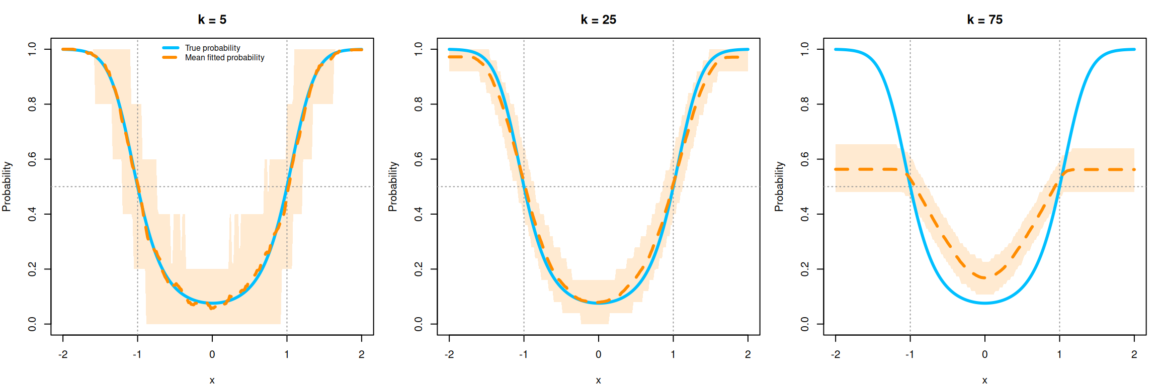
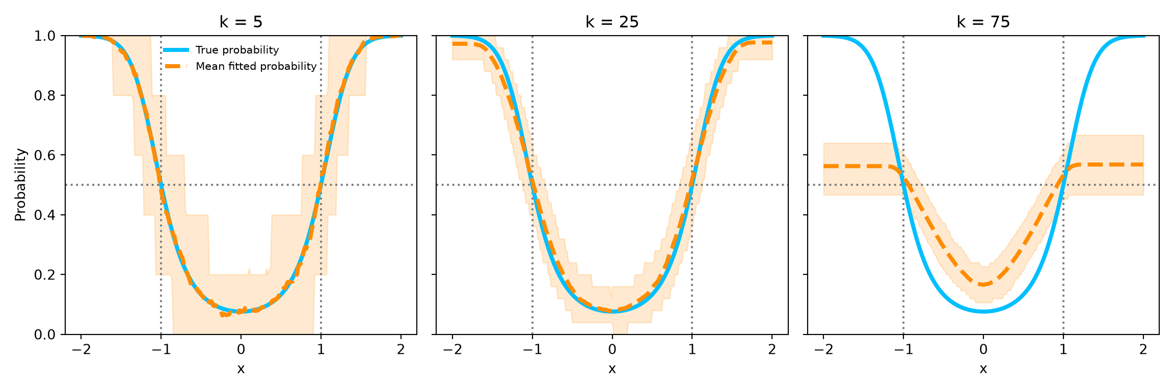
The blue curve is the true probability. The orange curve averages the fitted probabilities over training samples. The shaded band contains the middle 80 percent of the fitted probabilities at each location.¹

The gap between the orange and blue curves shows bias. The spread of fitted probabilities around their mean shows the training-sample variation measured by the variance term above.

R

old_par <- par(mfrow = c(1, 3), mar = c(4, 4, 3, 1))
for (k in c(5, 25, 75)) {
  j <- match(k, k_values)
  p_mean <- colMeans(p_hat[, , j])
  band <- apply(p_hat[, , j], 2, quantile, probs = c(0.1, 0.9))

  plot(x_grid, p_true, type = "n", ylim = c(0, 1),
       xlab = "x", ylab = "Probability", main = paste("k =", k))
  polygon(c(x_grid, rev(x_grid)), c(band[1, ], rev(band[2, ])),
          col = adjustcolor("darkorange", alpha.f = 0.18), border = NA)
  abline(h = 0.5, v = c(-1, 1), col = "gray60", lty = 3)
  lines(x_grid, p_true, col = "deepskyblue", lwd = 3)
  lines(x_grid, p_mean, col = "darkorange", lwd = 3, lty = 2)
  if (k == 5) {
    legend("top", c("True probability", "Mean fitted probability"),
           col = c("deepskyblue", "darkorange"), lty = c(1, 2),
           lwd = 3, bty = "n", cex = 0.75)
  }
}

True probabilities and variation in fitted KNN probabilities across 200 training samples.

par(old_par)

Python

fig, axes = plt.subplots(1, 3, figsize=(12, 4), sharey=True)
for ax, k in zip(axes, [5, 25, 75]):
    j = np.flatnonzero(k_values == k)[0]
    p_mean = p_hat[:, :, j].mean(axis=0)
    band = np.quantile(p_hat[:, :, j], [0.1, 0.9], axis=0)

    ax.fill_between(x_grid, band[0], band[1], color="darkorange", alpha=0.18)
    ax.axhline(0.5, color="gray", linestyle=":")
    for boundary in [-1, 1]:
        ax.axvline(boundary, color="gray", linestyle=":")
    ax.plot(x_grid, p_true, color="deepskyblue", linewidth=3,
            label="True probability")
    ax.plot(x_grid, p_mean, color="darkorange", linewidth=3,
            linestyle="--", label="Mean fitted probability")
    ax.set(xlabel="x", title=f"k = {k}", ylim=(0, 1))
axes[0].set_ylabel("Probability")
axes[0].legend(loc="upper center", frameon=False, fontsize=8)
fig.tight_layout()
plt.show()

True probabilities and variation in fitted KNN probabilities across 200 training samples.

At $k=5$, the fitted probabilities vary substantially across training samples. At $k=25$, the band is narrower and the mean curve still follows the changes near $x=-1$ and $x=1$. At $k=75$, averaging over broad neighborhoods washes out those changes. The result is lower variance but substantial smoothing bias.

Separate squared bias and variance

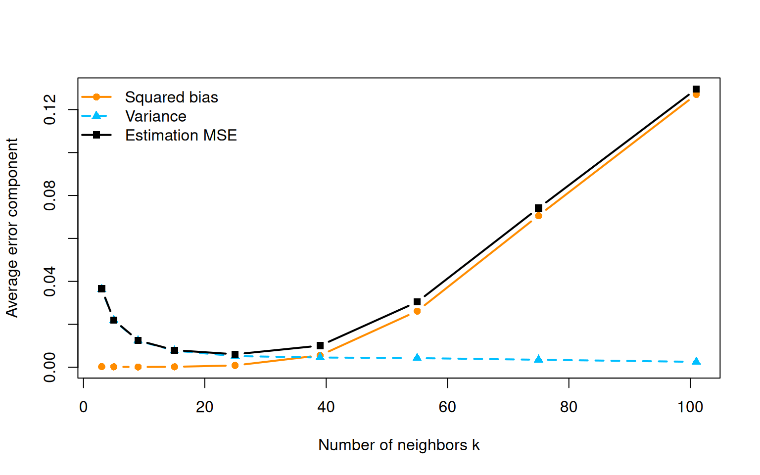
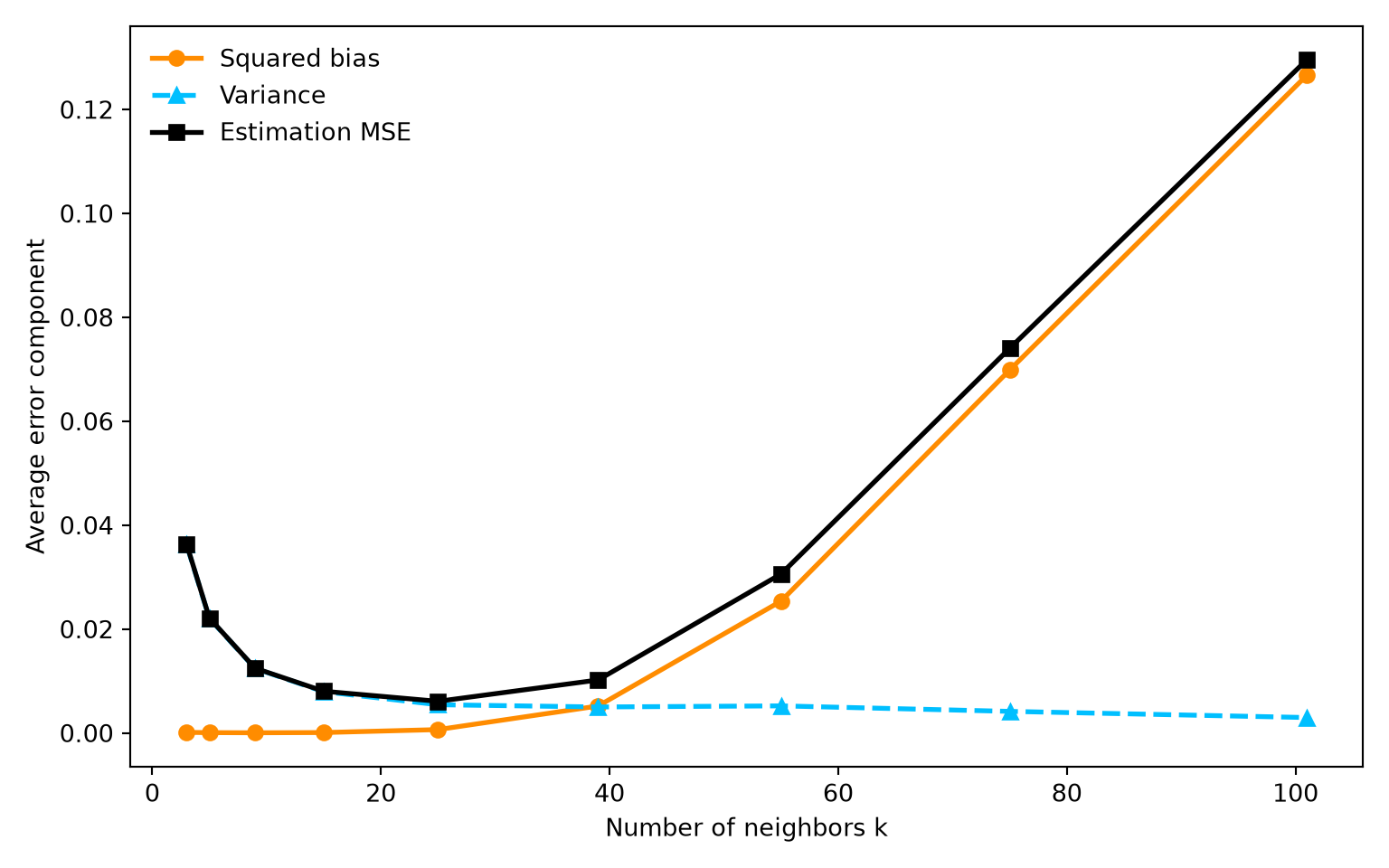
At every grid location, estimate squared bias from the mean fitted probability and estimate variance from the spread across repetitions. Then average these quantities over $x$ to summarize performance across the population.²

R

# Trapezoidal weights average over X ~ Uniform(-2, 2).
weights <- rep(1, length(x_grid))
weights[c(1, length(weights))] <- 0.5
weights <- weights / sum(weights)
bias2 <- variance <- mse <- numeric(length(k_values))

for (j in seq_along(k_values)) {
  p_mean <- colMeans(p_hat[, , j])
  bias2[j] <- sum(weights * (p_mean - p_true)^2)
  variance[j] <- sum(weights * colMeans(sweep(p_hat[, , j], 2, p_mean)^2))
  mse[j] <- sum(weights * colMeans(sweep(p_hat[, , j], 2, p_true)^2))
}

matplot(k_values, cbind(bias2, variance, mse), type = "b",
        col = c("darkorange", "deepskyblue", "black"),
        pch = c(16, 17, 15), lty = c(1, 2, 1), lwd = 2,
        xlab = "Number of neighbors k", ylab = "Average error component")
legend("topleft", c("Squared bias", "Variance", "Estimation MSE"),
       col = c("darkorange", "deepskyblue", "black"),
       pch = c(16, 17, 15), lty = c(1, 2, 1), lwd = 2, bty = "n")

Squared probability bias, variance, and their sum, averaged over the predictor distribution.

Python

# Trapezoidal weights average over X ~ Uniform(-2, 2).
weights = np.ones(len(x_grid))
weights[[0, -1]] = 0.5
weights /= weights.sum()
bias2 = np.empty(len(k_values))
variance = np.empty(len(k_values))
mse = np.empty(len(k_values))

for j in range(len(k_values)):
    p_mean = p_hat[:, :, j].mean(axis=0)
    bias2[j] = weights @ (p_mean - p_true)**2
    variance[j] = weights @ ((p_hat[:, :, j] - p_mean)**2).mean(axis=0)
    mse[j] = weights @ ((p_hat[:, :, j] - p_true)**2).mean(axis=0)

plt.figure(figsize=(8, 5))
plt.plot(k_values, bias2, "o-", color="darkorange", linewidth=2,
         label="Squared bias")
plt.plot(k_values, variance, "^--", color="deepskyblue", linewidth=2,
         label="Variance")
plt.plot(k_values, mse, "s-", color="black", linewidth=2,
         label="Estimation MSE")
plt.xlabel("Number of neighbors k")
plt.ylabel("Average error component")
plt.legend(frameon=False)
plt.tight_layout()
plt.show()

Squared probability bias, variance, and their sum, averaged over the predictor distribution.

The estimated variance generally falls as neighborhoods become larger. Squared bias rises sharply for large neighborhoods. Their sum is smallest at a moderate $k$. The irreducible Brier component, averaged over $X$, is about $0.109$ for every $k$. Adding it shifts the entire MSE curve upward without changing which $k$ is best in this comparison.

How probability error becomes classification error

Recall the opening examples: estimates of $0.49$ and $0.51$ give different decisions, while $0.60$ and $0.95$ give the same decision. This is why the squared-loss decomposition does not carry over directly to $0$-$1$ loss. A probability error changes a decision only if it moves the estimate across the cutoff.

Fix a decision rule $d$. At a particular $x$, agreeing with the Bayes decision adds no error. If $p(x)\geq 1/2$ but $d(x)=0$, the extra conditional error is

$$p(x)-\{1-p(x)\}=2p(x)-1.$$

If $p(x)<1/2$ but $d(x)=1$, it is $1-2p(x)$. Combining these cases and averaging gives

$$\boxed{R(d)-R^*=E\left[|2p(X)-1|\,I\{d(X)\neq d^*(X)\}\right].}$$

This is the excess classification error: the error above the Bayes benchmark. It depends on where the classifier disagrees with the Bayes rule and how costly each disagreement is.

• Near $p(x)=1/2$, a small probability change can reverse the decision, but the extra error from that reversal is small.
• Far from $1/2$, reversing the decision requires a larger probability error, and the extra error is larger.

For example, predicting class 0 when $p(x)=0.52$ adds $0.04$ to the conditional error. Making the same decision when $p(x)=0.90$ adds $0.80$.

Return to the KNN experiment

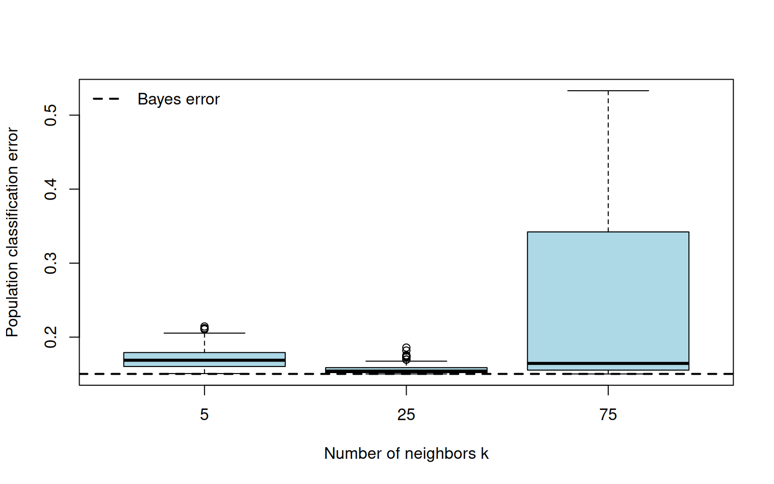
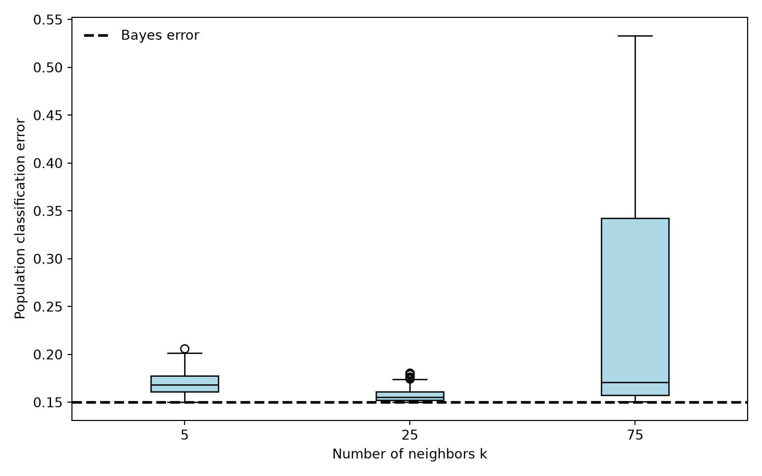
Because we know $p(x)$ in the simulation, we can calculate each fitted rule’s conditional error directly: use $p(x)$ where it predicts 0 and $1-p(x)$ where it predicts 1. Averaging over the grid approximates population classification error. This isolates variation caused by the training sample without adding random test outcomes.

R

bayes_error <- sum(weights * pmin(p_true, 1 - p_true))
error <- matrix(NA_real_, repetitions, length(k_values))
for (j in seq_along(k_values)) {
  for (r in seq_len(repetitions)) {
    predicted <- p_hat[r, , j] >= 0.5
    error[r, j] <- sum(weights * ifelse(predicted, 1 - p_true, p_true))
  }
}
round(bayes_error, 3)

[1] 0.15

boxplot(error[, match(c(5, 25, 75), k_values)], names = c(5, 25, 75),
        col = "lightblue", ylim = range(c(bayes_error, error)),
        xlab = "Number of neighbors k", ylab = "Population classification error")
abline(h = bayes_error, lty = 2, lwd = 2)
legend("topleft", "Bayes error", lty = 2, lwd = 2, bty = "n")

Approximate population classification errors across 200 fitted KNN models. The dashed line is the Bayes error.

Python

bayes_error = weights @ np.minimum(p_true, 1 - p_true)
error = np.empty((repetitions, len(k_values)))
for j in range(len(k_values)):
    for r in range(repetitions):
        predicted = p_hat[r, :, j] >= 0.5
        error[r, j] = weights @ np.where(predicted, 1 - p_true, p_true)
print(round(bayes_error, 3))

0.15

plt.figure(figsize=(8, 5))
plt.boxplot([error[:, np.flatnonzero(k_values == k)[0]] for k in [5, 25, 75]],
            tick_labels=[5, 25, 75], patch_artist=True,
            boxprops={"facecolor": "lightblue"},
            medianprops={"color": "black"})
plt.axhline(bayes_error, color="black", linestyle="--", linewidth=2,
            label="Bayes error")
plt.xlabel("Number of neighbors k")
plt.ylabel("Population classification error")
plt.legend(loc="upper left", frameon=False)
plt.tight_layout()
plt.show()

Approximate population classification errors across 200 fitted KNN models. The dashed line is the Bayes error.

The Bayes error is about $0.150$. At $k=5$, fitted probabilities fluctuate because each estimate uses few observations. At $k=25$, the fitted curves follow the population pattern more closely. At $k=75$, strong smoothing puts a broad part of the mean fitted curve near $1/2$, so changes in the training sample can move many decisions across the cutoff.

Lower probability variance therefore does not guarantee more stable class decisions. Its effect depends on where the fitted probabilities lie relative to the cutoff.

Unequal error costs

So far, false positives and false negatives have equal cost. Suppose instead that a false positive costs $c_{\mathrm{FP}}>0$, a false negative costs $c_{\mathrm{FN}}>0$, and correct decisions have zero cost.

We repeat the Bayes comparison of the two possible decisions, now using these costs in place of $0$-$1$ loss.

At a fixed $x$, predicting 1 has expected cost $c_{\mathrm{FP}}\{1-p(x)\}$, while predicting 0 has expected cost $c_{\mathrm{FN}}p(x)$. Choose class 1 when

$$c_{\mathrm{FP}}\{1-p(x)\}\leq c_{\mathrm{FN}}p(x),$$

or equivalently when

$$\boxed{p(x)\geq\frac{c_{\mathrm{FP}}}{c_{\mathrm{FP}}+c_{\mathrm{FN}}}.}$$

If a false negative costs four times as much as a false positive, the cutoff is $1/5$. We accept more positive decisions because missing a positive case is more costly. In practice, we substitute an estimated probability and examine the consequences of the chosen cutoff. That is the subject of the next lecture.

A note on imbalanced classes

Class imbalance alone does not change the Bayes cutoff under equal error costs when $p(x)$ is the conditional probability in the population of interest. Those probabilities already reflect the class prevalence. A different cutoff follows from different costs or a different decision objective. If training observations were deliberately sampled to change the class proportions, the fitted probabilities may need adjustment before applying a probability-based decision rule.

Check your understanding

1. If $p(x)=0.7$, what is the Bayes decision and its conditional error? What changes if we estimate this probability by $0.9$?
2. Why are the irreducible Brier loss and Bayes classification error different?
3. How do the KNN probability bands and bias-variance curves explain the effect of increasing $k$?
4. Why can a low-variance probability estimate still produce unstable class decisions?
5. What happens to the optimal cutoff when false negatives become more costly?

Key ideas

1. A probability estimate and a class decision are different predictions.
2. The Bayes classifier minimizes expected $0$-$1$ loss, but overlapping classes still create errors.
3. Brier loss and log loss reward accurate probabilities. Squared probability error has the familiar bias-variance decomposition.
4. Classification error depends on whether probability errors change the decision and how far the true probability lies from the cutoff.
5. The costs of the two kinds of error determine the appropriate decision rule.

Next: use logistic probabilities to study confusion matrices, cutoffs, and ROC curves.

References and further reading

• James, G., Witten, D., Hastie, T., Tibshirani, R., and Taylor, J. (2023). An Introduction to Statistical Learning, Chapters 2 and 4. Springer.
• Hastie, T., Tibshirani, R., and Friedman, J. (2009). The Elements of Statistical Learning, Chapters 2 and 4. Springer.

Footnotes

1. This is a pointwise description of variation across fitted models, not a confidence band for the true probability curve.

2. The equally spaced grid and half weights at its endpoints implement the trapezoidal rule for the uniform predictor distribution. For the finite simulation, variance uses the number of repetitions as its divisor, so the calculated MSE equals squared bias plus variance exactly. These remain Monte Carlo estimates of the corresponding population quantities.