Skip to main content

Fixed-Design Prediction Error and Model Selection

Theory and simulation

On this page

• Learning goals
• Why training error is not enough
• A simulation study
• Why training and test error differ on average
• From optimism to Mallows’ $C_p$
• AIC, BIC, and validation
• Check your understanding
• Key ideas
• References and further reading

← Week 2 overview · Continue to the implementation lecture →

Adding covariates always improves the fit to the training data. Does it also improve prediction? We begin with two simple simulations, explain their behavior using fixed-design prediction error, and use the result to motivate Mallows’ $C_p$.

Learning goals

By the end of this lecture, you should be able to:

• explain why training error alone favors larger nested least-squares models;
• use simulation to identify the bias-variance trade-off in prediction;
• derive expected training and test MSE for a fixed design; and
• explain how their difference motivates Mallows’ $C_p$, AIC, and BIC.

Why training error is not enough

A larger least-squares model can always fit the training data at least as well as a smaller nested model. If training error were our only score, there would be no reason to stop before using every available covariate. The difficulty is that a new covariate can improve the fit for two very different reasons:

1. it may explain genuine structure in the mean response; or
2. it may happen to align with noise in this particular sample.

Only the first improvement is reliably useful for prediction. The second makes the fitted model look better on the data it has already seen, but that accidental pattern will not generally repeat.

Guiding question. How can we estimate prediction error when the training error we observe is too small on average?

We will answer this in three stages: first make the problem visible in a simulation where the truth is known, then explain the curves with projection geometry, and finally use that explanation to construct model-selection criteria for real data.

A simulation study

We begin with a simple question: what happens when we keep adding covariates to a linear regression? We answer it in a setting where the truth is known.

Generate one covariate matrix with $n=100$ observations, $p=20$ available covariates, and independent standard normal entries,

$$\mathbf X_{\mathrm{all}}=(\mathbf x_1,\ldots,\mathbf x_p) \in\mathbb R^{n\times p}, \qquad (\mathbf X_{\mathrm{all}})_{ij}\stackrel{\mathrm{iid}}{\sim}N(0,1).$$

Add an intercept column to form the full design matrix:

$$\mathbf X=[\mathbf 1,\mathbf X_{\mathrm{all}}] \in\mathbb R^{n\times(p+1)}, \qquad \boldsymbol\beta=(\beta_0,\beta_1,\ldots,\beta_p)^{\mathsf T}.$$

Thus, $p$ counts the covariates and $p+1$ counts all coefficients, including the intercept. We keep this realized design fixed across all simulation repetitions. The candidate model indexed by $m$ uses the first $m$ covariates and an intercept:

$$\mathbf X_m=[\mathbf 1,\mathbf x_1,\ldots,\mathbf x_m] \in\mathbb R^{n\times(m+1)}.$$

A candidate with $m$ covariates has $m+1$ fitted coefficients, including the intercept. We use $i$ for observations and $j$ for covariates; $m$ indexes candidate size and $k$ indexes simulation repetitions in the code.

Draw a pair of independent error vectors and construct two responses at the same covariate values:

$$\begin{aligned} \mathbf y &= \mathbf X\boldsymbol\beta+\boldsymbol\epsilon,\\ \mathbf y^* &= \mathbf X\boldsymbol\beta+\boldsymbol\epsilon^*, \end{aligned}$$

where $\mathbf X\boldsymbol\beta$ is the true mean response in both cases. We will choose $\boldsymbol\beta$ in two ways below. For these simulations,

$$\boldsymbol\epsilon,\boldsymbol\epsilon^* \stackrel{\mathrm{ind}}{\sim} \mathcal N_n(\mathbf 0,\mathbf I_n).$$

Here $\mathbf I_n$ is the $100\times100$ identity matrix, and every error has variance $\sigma^2=1$. Repeat this experiment 1,000 times, drawing fresh independent errors each time. Within each repetition, fit every candidate model using the same $\mathbf y$, then calculate its training MSE from $\mathbf y$ and its test MSE from the same independent response $\mathbf y^*$. Thus, model sizes are compared on one response pair, while a fresh pair is generated for every repetition.

Repeating the experiment 1,000 times estimates the expected training and test MSE conditional on the fixed design. Throughout this lecture, prediction error means expected test MSE. One realized training/test response pair produces only one observed test-MSE curve, which need not vary smoothly across the candidate models.

The R setup below generates and saves only the fixed covariate matrix so that Python uses the same $\mathbf X_{\mathrm{all}}$. Each language draws fresh errors inside every simulation repetition and uses a fixed seed to make its own simulation reproducible. Because R and Python use different random-number generators, their Monte Carlo curves need not be numerically identical, but both should track the same theoretical expectations.

R and Python implementations

R

# Generate the fixed covariate matrix used in every simulation repetition.
set.seed(432)
n <- 100
p <- 20
nsim <- 1000
sigma <- 1
X_all <- matrix(rnorm(n * p), nrow = n, ncol = p)
X <- cbind(1, X_all)
covariate_count <- 0:p

# Save the fixed covariate matrix as a bridge from R to Python.
colnames(X_all) <- paste0("x", 1:p)
write.csv(X_all, "data/week-02/fixed-x.csv", row.names = FALSE)

Python

import numpy as np
import pandas as pd
import matplotlib.pyplot as plt

# Use the fixed covariate matrix generated in the R setup above.
X_all = pd.read_csv("data/week-02/fixed-x.csv").to_numpy()

n, p = X_all.shape
X = np.column_stack((np.ones(n), X_all))
nsim = 1000
sigma = 1.0

covariate_count = np.arange(p + 1)

Predict before viewing the curves.

Make three predictions.

1. Because each larger model contains the previous model, what must happen to training MSE?
2. If an added covariate mainly captures a random fluctuation in the training response, should the same apparent improvement occur for the independent test response?
3. Once a model can already describe all of the systematic signal, what useful work remains for another covariate to do?

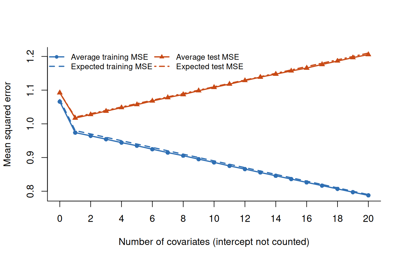
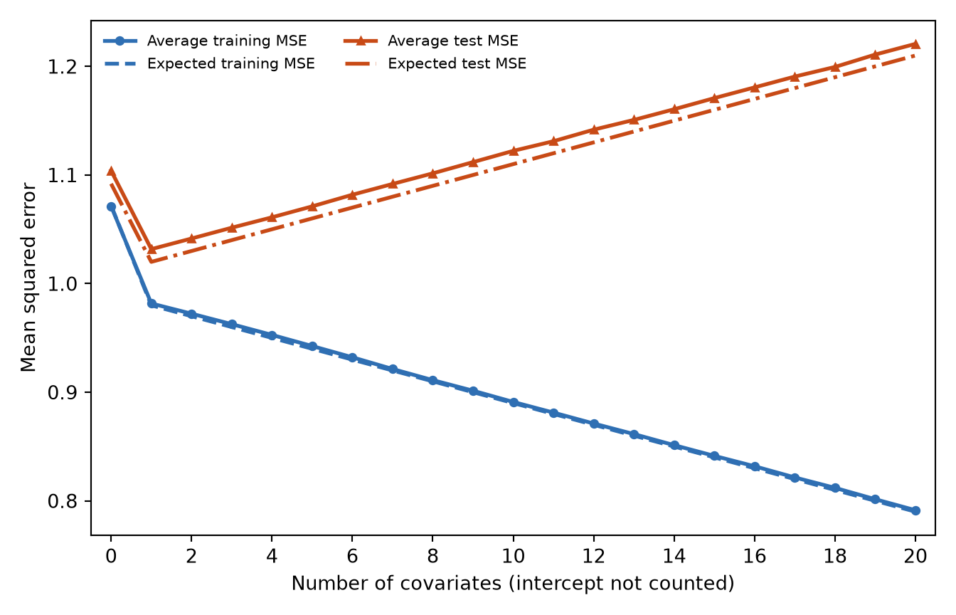
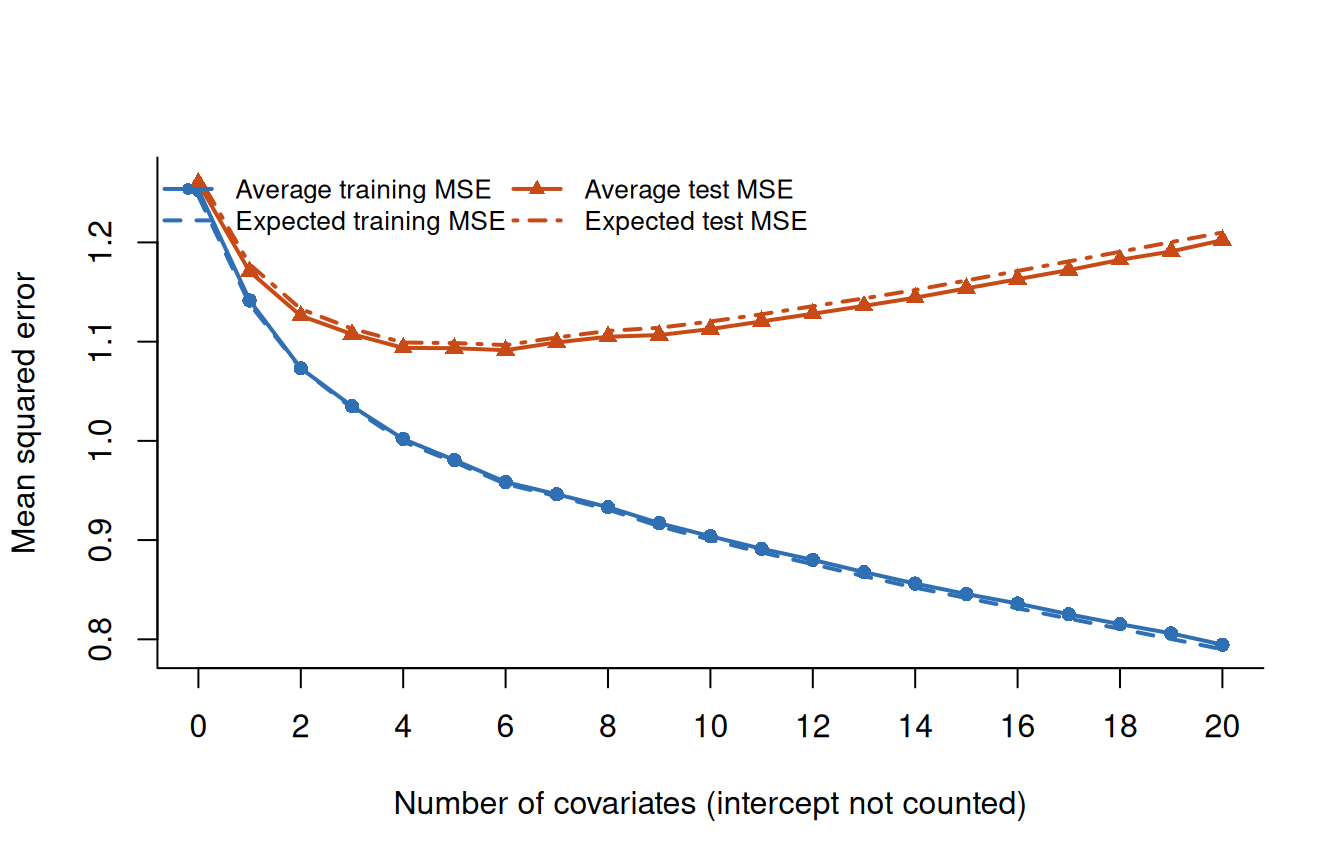
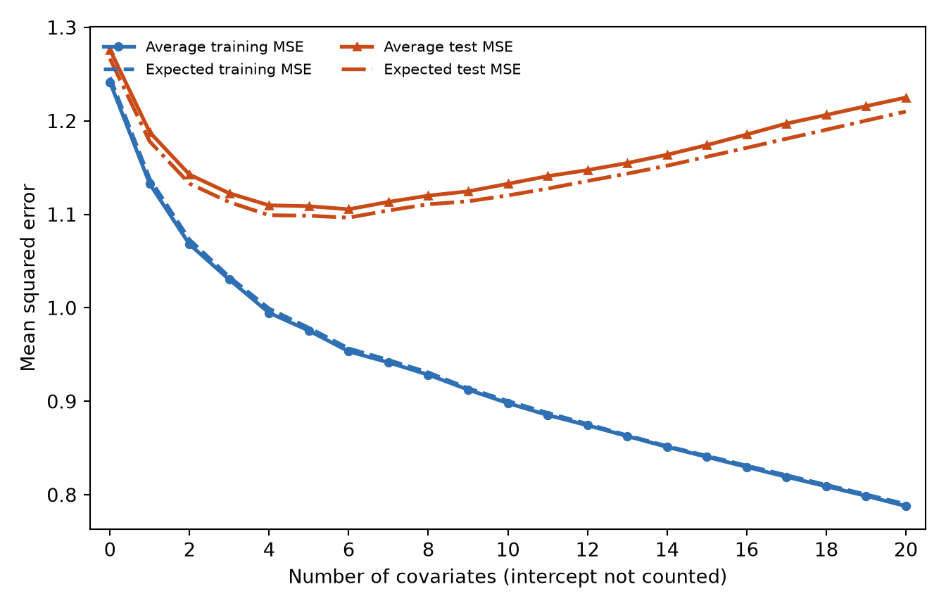
The plots use blue circles for average simulated training MSE and orange triangles for average simulated test MSE. The theoretical training curve is dashed, while the theoretical test curve is dot-dashed. A curve from one realized training/test response pair would be noisier and need not move smoothly.

Scenario 1: one useful covariate

First set

$$\boldsymbol\beta=(0,0.3,0,\ldots,0)^{\mathsf T} \in\mathbb R^{p+1}, \qquad \mathbf X\boldsymbol\beta=0.3\mathbf x_1.$$

The intercept coefficient $\beta_0$ is zero, and only $\beta_1$ is nonzero. The systematic mean response is therefore proportional to the first covariate column, $\mathbf x_1$. Once covariate $X_1$ enters the model, all of that signal is included. Later covariates do not add any new mean structure.

R

beta <- c(0, 0.3, rep(0, p - 1))
train_mse_one <- matrix(NA_real_, nrow = nsim, ncol = p + 1)
test_mse_one <- matrix(NA_real_, nrow = nsim, ncol = p + 1)

set.seed(433)
for (k in seq_len(nsim)) {
  # Generate fresh independent training and test responses.
  y_train <- drop(X %*% beta) + rnorm(n, sd = sigma)
  y_test <- drop(X %*% beta) + rnorm(n, sd = sigma)

  # Use this response pair for every candidate model in this repetition.
  y_hat <- rep(mean(y_train), n)
  train_mse_one[k, 1] <- mean((y_train - y_hat)^2)
  test_mse_one[k, 1] <- mean((y_test - y_hat)^2)

  # Continue with nested models using the first m covariates.
  for (m in 1:p) {
    train_data <- data.frame(y = y_train, X_all[, 1:m, drop = FALSE])
    test_data <- data.frame(X_all[, 1:m, drop = FALSE])

    fit <- lm(y ~ ., data = train_data)
    y_hat <- predict(fit, newdata = test_data)

    train_mse_one[k, m + 1] <- mean(residuals(fit)^2)
    test_mse_one[k, m + 1] <- mean((y_test - y_hat)^2)
  }
}

mean_train_mse_one <- colMeans(train_mse_one)
mean_test_mse_one <- colMeans(test_mse_one)

# Calculate the approximation bias for each candidate model.
bias_mse_one <- numeric(p + 1)
bias_mse_one[1] <- mean((drop(X %*% beta) - mean(X %*% beta))^2)

for (m in 1:p) {
  mean_data <- data.frame(y = drop(X %*% beta), X_all[, 1:m, drop = FALSE])
  mean_fit <- lm(y ~ ., data = mean_data)
  bias_mse_one[m + 1] <- mean(residuals(mean_fit)^2)
}

theory_train_mse_one <- bias_mse_one +
  (1 - (covariate_count + 1) / n) * sigma^2
theory_test_mse_one <- bias_mse_one +
  (1 + (covariate_count + 1) / n) * sigma^2

train_color <- "#2F6FB3"
test_color <- "#C84A16"

# Compare the Monte Carlo averages with their theoretical expectations.
y_limits <- range(
  mean_train_mse_one, mean_test_mse_one,
  theory_train_mse_one, theory_test_mse_one
)

par(bty = "l")
plot(
  covariate_count, mean_train_mse_one,
  type = "o", pch = 16, col = train_color, lwd = 2,
  xlab = "Number of covariates (intercept not counted)",
  ylab = "Mean squared error", ylim = y_limits,
  xaxt = "n"
)
axis(1, at = seq(0, p, by = 2))
lines(covariate_count, theory_train_mse_one,
      col = train_color, lwd = 2, lty = 2)
lines(covariate_count, mean_test_mse_one,
      type = "o", pch = 17, col = test_color, lwd = 2)
lines(covariate_count, theory_test_mse_one,
      col = test_color, lwd = 2, lty = 4)
legend(
  "topleft",
  legend = c(
    "Average training MSE", "Expected training MSE",
    "Average test MSE", "Expected test MSE"
  ),
  col = c(train_color, train_color, test_color, test_color),
  lty = c(1, 2, 1, 4), pch = c(16, NA, 17, NA),
  lwd = 2, bty = "n", ncol = 2, cex = 0.82
)

Average training and test MSE when only X1 carries signal. Blue circles identify average simulated training MSE and orange triangles identify average simulated test MSE. Dashed and dot-dashed curves are the corresponding theoretical expectations.

Python

beta = np.zeros(p + 1)
beta[1] = 0.3
train_mse_one = np.empty((nsim, p + 1))
test_mse_one = np.empty((nsim, p + 1))

rng_one = np.random.default_rng(433)
for k in range(nsim):
    # Generate fresh independent training and test responses.
    y_train = X @ beta + rng_one.normal(loc=0.0, scale=sigma, size=n)
    y_test = X @ beta + rng_one.normal(loc=0.0, scale=sigma, size=n)

    # Use this response pair for every candidate model in this repetition.
    y_hat = np.repeat(y_train.mean(), n)
    train_mse_one[k, 0] = np.mean((y_train - y_hat) ** 2)
    test_mse_one[k, 0] = np.mean((y_test - y_hat) ** 2)

    # Continue with nested models using the first m covariates.
    for m in range(1, p + 1):
        X_m = X[:, :m + 1]
        beta_hat = np.linalg.lstsq(X_m, y_train, rcond=None)[0]
        y_hat = X_m @ beta_hat

        train_mse_one[k, m] = np.mean((y_train - y_hat) ** 2)
        test_mse_one[k, m] = np.mean((y_test - y_hat) ** 2)

mean_train_mse_one = train_mse_one.mean(axis=0)
mean_test_mse_one = test_mse_one.mean(axis=0)

# Calculate the approximation bias for each candidate model.
bias_mse_one = np.empty(p + 1)
bias_mse_one[0] = np.mean((X @ beta - (X @ beta).mean()) ** 2)

for m in range(1, p + 1):
    X_m = X[:, :m + 1]
    beta_hat = np.linalg.lstsq(X_m, X @ beta, rcond=None)[0]
    y_hat = X_m @ beta_hat
    bias_mse_one[m] = np.mean((X @ beta - y_hat) ** 2)

theory_train_mse_one = bias_mse_one + \
    (1 - (covariate_count + 1) / n) * sigma**2
theory_test_mse_one = bias_mse_one + \
    (1 + (covariate_count + 1) / n) * sigma**2

train_color = "#2F6FB3"
test_color = "#C84A16"

# Compare the Monte Carlo averages with their theoretical expectations.
plt.figure(figsize=(7, 4.5))
plt.plot(covariate_count, mean_train_mse_one, "o-", color=train_color,
         linewidth=2, markersize=4, label="Average training MSE")
plt.plot(covariate_count, theory_train_mse_one, "--", color=train_color,
         linewidth=2, label="Expected training MSE")
plt.plot(covariate_count, mean_test_mse_one, "^-", color=test_color,
         linewidth=2, markersize=4, label="Average test MSE")
plt.plot(covariate_count, theory_test_mse_one, "-.", color=test_color,
         linewidth=2, label="Expected test MSE")
plt.xlabel("Number of covariates (intercept not counted)")
plt.ylabel("Mean squared error")
plt.xticks(np.arange(0, p + 1, 2))

([<matplotlib.axis.XTick object at 0x7ff998ab1290>, <matplotlib.axis.XTick object at 0x7ff998d0e410>, <matplotlib.axis.XTick object at 0x7ff998a79350>, <matplotlib.axis.XTick object at 0x7ff998b0f410>, <matplotlib.axis.XTick object at 0x7ff998b10ad0>, <matplotlib.axis.XTick object at 0x7ff998b12950>, <matplotlib.axis.XTick object at 0x7ff998b18910>, <matplotlib.axis.XTick object at 0x7ff998b1a7d0>, <matplotlib.axis.XTick object at 0x7ff998b24810>, <matplotlib.axis.XTick object at 0x7ff998ff3d50>, <matplotlib.axis.XTick object at 0x7ff998b26790>], [Text(0, 0, '0'), Text(2, 0, '2'), Text(4, 0, '4'), Text(6, 0, '6'), Text(8, 0, '8'), Text(10, 0, '10'), Text(12, 0, '12'), Text(14, 0, '14'), Text(16, 0, '16'), Text(18, 0, '18'), Text(20, 0, '20')])

plt.xlim(-0.5, p + 0.5)

(-0.5, 20.5)

plt.legend(frameon=False, ncol=2, fontsize=8, loc="upper left")
plt.tight_layout()
plt.show()

Average training and test MSE when only X1 carries signal. Blue circles identify average simulated training MSE and orange triangles identify average simulated test MSE. Dashed and dot-dashed curves are the corresponding theoretical expectations.

The drop from zero to one covariate has a different explanation from everything that follows. The intercept-only model leaves the systematic pattern from $X_1$ unexplained. Adding $X_1$ captures that pattern, so both training and test MSE fall. After $X_1$ is included, later covariates cannot recover any missing signal.

Why, then, does the blue curve keep falling? A later covariate can happen to align with a random fluctuation in the training response, and least squares uses that alignment to improve the in-sample fit. The independent test response contains different noise, so the fitted noise pattern is not reliably useful there. Training MSE therefore keeps falling, while average test MSE rises.

The dashed curves preview an exact result that we will derive. Here $n=100$ and $\sigma^2=1$, and each later covariate adds one fitted coefficient. On average, that coefficient lowers expected training MSE by $1/100=0.01$, raises expected test MSE by $0.01$, and therefore widens their gap by $0.02$. A single realized dataset need not change by exactly these amounts; the calculation describes the average over fresh training/test response pairs at the fixed design.

Scenario 2: a gradually decaying signal

Now let the coefficients decrease gradually across the ordered covariates:

$$\beta_0=0, \qquad \beta_j=0.4^{\sqrt{j}}, \quad j=1,\ldots,p.$$

The response model is still $\mathbf y=\mathbf X\boldsymbol\beta+\boldsymbol\epsilon$, with $p+1$ coefficients including the intercept. The first covariate has coefficient $0.4$, the fourth has coefficient $0.16$, and later covariates have progressively smaller effects.

The early covariates therefore carry more signal, while the later covariates are not exactly useless. The construction is designed so that moving to the right along the nested sequence tends to recover progressively smaller amounts of the remaining signal. This lets us see when the remaining benefit of another fitted coefficient is no longer large enough to offset its added variability.

R

beta <- c(0, 0.4^sqrt(1:p))
train_mse_decay <- matrix(NA_real_, nrow = nsim, ncol = p + 1)
test_mse_decay <- matrix(NA_real_, nrow = nsim, ncol = p + 1)

set.seed(434)
for (k in seq_len(nsim)) {
  # Generate fresh independent training and test responses.
  y_train <- drop(X %*% beta) + rnorm(n, sd = sigma)
  y_test <- drop(X %*% beta) + rnorm(n, sd = sigma)

  # Use this response pair for every candidate model in this repetition.
  y_hat <- rep(mean(y_train), n)
  train_mse_decay[k, 1] <- mean((y_train - y_hat)^2)
  test_mse_decay[k, 1] <- mean((y_test - y_hat)^2)

  # Continue with nested models using the first m covariates.
  for (m in 1:p) {
    train_data <- data.frame(y = y_train, X_all[, 1:m, drop = FALSE])
    test_data <- data.frame(X_all[, 1:m, drop = FALSE])

    fit <- lm(y ~ ., data = train_data)
    y_hat <- predict(fit, newdata = test_data)

    train_mse_decay[k, m + 1] <- mean(residuals(fit)^2)
    test_mse_decay[k, m + 1] <- mean((y_test - y_hat)^2)
  }
}

mean_train_mse_decay <- colMeans(train_mse_decay)
mean_test_mse_decay <- colMeans(test_mse_decay)

# Calculate the approximation bias for each candidate model.
bias_mse_decay <- numeric(p + 1)
bias_mse_decay[1] <- mean((drop(X %*% beta) - mean(X %*% beta))^2)

for (m in 1:p) {
  mean_data <- data.frame(y = drop(X %*% beta), X_all[, 1:m, drop = FALSE])
  mean_fit <- lm(y ~ ., data = mean_data)
  bias_mse_decay[m + 1] <- mean(residuals(mean_fit)^2)
}

theory_train_mse_decay <- bias_mse_decay +
  (1 - (covariate_count + 1) / n) * sigma^2
theory_test_mse_decay <- bias_mse_decay +
  (1 + (covariate_count + 1) / n) * sigma^2

# Compare the Monte Carlo averages with their theoretical expectations.
y_limits <- range(
  mean_train_mse_decay, mean_test_mse_decay,
  theory_train_mse_decay, theory_test_mse_decay
)

par(bty = "l")
plot(
  covariate_count, mean_train_mse_decay,
  type = "o", pch = 16, col = train_color, lwd = 2,
  xlab = "Number of covariates (intercept not counted)",
  ylab = "Mean squared error", ylim = y_limits,
  xaxt = "n"
)
axis(1, at = seq(0, p, by = 2))
lines(covariate_count, theory_train_mse_decay,
      col = train_color, lwd = 2, lty = 2)
lines(covariate_count, mean_test_mse_decay,
      type = "o", pch = 17, col = test_color, lwd = 2)
lines(covariate_count, theory_test_mse_decay,
      col = test_color, lwd = 2, lty = 4)
legend(
  "topleft",
  legend = c(
    "Average training MSE", "Expected training MSE",
    "Average test MSE", "Expected test MSE"
  ),
  col = c(train_color, train_color, test_color, test_color),
  lty = c(1, 2, 1, 4), pch = c(16, NA, 17, NA),
  lwd = 2, bty = "n", ncol = 2, cex = 0.82
)

Average training and test MSE under a decaying coefficient sequence. Blue circles identify average simulated training MSE and orange triangles identify average simulated test MSE. Dashed and dot-dashed curves are the corresponding theoretical expectations.

Python

beta = np.zeros(p + 1)
beta[1:] = 0.4 ** np.sqrt(np.arange(1, p + 1))
train_mse_decay = np.empty((nsim, p + 1))
test_mse_decay = np.empty((nsim, p + 1))

rng_decay = np.random.default_rng(434)
for k in range(nsim):
    # Generate fresh independent training and test responses.
    y_train = X @ beta + rng_decay.normal(loc=0.0, scale=sigma, size=n)
    y_test = X @ beta + rng_decay.normal(loc=0.0, scale=sigma, size=n)

    # Use this response pair for every candidate model in this repetition.
    y_hat = np.repeat(y_train.mean(), n)
    train_mse_decay[k, 0] = np.mean((y_train - y_hat) ** 2)
    test_mse_decay[k, 0] = np.mean((y_test - y_hat) ** 2)

    # Continue with nested models using the first m covariates.
    for m in range(1, p + 1):
        X_m = X[:, :m + 1]
        beta_hat = np.linalg.lstsq(X_m, y_train, rcond=None)[0]
        y_hat = X_m @ beta_hat

        train_mse_decay[k, m] = np.mean((y_train - y_hat) ** 2)
        test_mse_decay[k, m] = np.mean((y_test - y_hat) ** 2)

mean_train_mse_decay = train_mse_decay.mean(axis=0)
mean_test_mse_decay = test_mse_decay.mean(axis=0)

# Calculate the approximation bias for each candidate model.
bias_mse_decay = np.empty(p + 1)
bias_mse_decay[0] = np.mean((X @ beta - (X @ beta).mean()) ** 2)

for m in range(1, p + 1):
    X_m = X[:, :m + 1]
    beta_hat = np.linalg.lstsq(X_m, X @ beta, rcond=None)[0]
    y_hat = X_m @ beta_hat
    bias_mse_decay[m] = np.mean((X @ beta - y_hat) ** 2)

theory_train_mse_decay = bias_mse_decay + \
    (1 - (covariate_count + 1) / n) * sigma**2
theory_test_mse_decay = bias_mse_decay + \
    (1 + (covariate_count + 1) / n) * sigma**2

# Compare the Monte Carlo averages with their theoretical expectations.
plt.figure(figsize=(7, 4.5))
plt.plot(covariate_count, mean_train_mse_decay, "o-", color=train_color,
         linewidth=2, markersize=4, label="Average training MSE")
plt.plot(covariate_count, theory_train_mse_decay, "--", color=train_color,
         linewidth=2, label="Expected training MSE")
plt.plot(covariate_count, mean_test_mse_decay, "^-", color=test_color,
         linewidth=2, markersize=4, label="Average test MSE")
plt.plot(covariate_count, theory_test_mse_decay, "-.", color=test_color,
         linewidth=2, label="Expected test MSE")
plt.xlabel("Number of covariates (intercept not counted)")
plt.ylabel("Mean squared error")
plt.xticks(np.arange(0, p + 1, 2))

([<matplotlib.axis.XTick object at 0x7ff998b36250>, <matplotlib.axis.XTick object at 0x7ff995942490>, <matplotlib.axis.XTick object at 0x7ff99e0c7250>, <matplotlib.axis.XTick object at 0x7ff995988910>, <matplotlib.axis.XTick object at 0x7ff99598a550>, <matplotlib.axis.XTick object at 0x7ff99598c490>, <matplotlib.axis.XTick object at 0x7ff99598e410>, <matplotlib.axis.XTick object at 0x7ff99598fe90>, <matplotlib.axis.XTick object at 0x7ff998b6be10>, <matplotlib.axis.XTick object at 0x7ff9959958d0>, <matplotlib.axis.XTick object at 0x7ff995997d50>], [Text(0, 0, '0'), Text(2, 0, '2'), Text(4, 0, '4'), Text(6, 0, '6'), Text(8, 0, '8'), Text(10, 0, '10'), Text(12, 0, '12'), Text(14, 0, '14'), Text(16, 0, '16'), Text(18, 0, '18'), Text(20, 0, '20')])

plt.xlim(-0.5, p + 0.5)

(-0.5, 20.5)

plt.legend(frameon=False, ncol=2, fontsize=8, loc="upper left")
plt.tight_layout()
plt.show()

Average training and test MSE under a decaying coefficient sequence. Blue circles identify average simulated training MSE and orange triangles identify average simulated test MSE. Dashed and dot-dashed curves are the corresponding theoretical expectations.

At first, adding a covariate recovers enough previously omitted signal to offset the extra variability created by estimating another coefficient, so average test MSE falls. Farther along the sequence, little signal remains to be recovered. The added fitting variability then exceeds the benefit, and average test MSE begins to rise. For this fixed design, the theoretical expected test MSE is minimized at six covariates, or seven fitted coefficients after counting the intercept. The two Monte Carlo curves fluctuate around that expectation because R and Python use separate error draws.

This pattern is a concrete example of the bias-variance trade-off, but it does not imply that every curve of average test MSE must be U-shaped. With strong signal in later covariates, average test MSE could continue falling. If none of the candidate covariates were useful, it could rise immediately. The shape depends on this particular signal and this particular fixed design.

One caution matters when covariates are correlated: a coefficient’s size alone does not tell us exactly how much signal its covariate adds. What matters is how much of the mean remains unexplained by the current model. The projection argument in the next section makes this idea precise.

Why training and test error differ on average

The simulations show the phenomenon. We now explain it for one candidate model whose covariate columns are fixed before observing the response.

For the derivation, we simplify the count: from here through the model-selection criteria, $p$ denotes the total number of columns in the candidate design matrix, including the intercept column if present. The projection argument treats every column in the same way, so we no longer count the intercept separately. A simulation candidate with $m$ covariates and an intercept therefore has $p=m+1$ in the formulas below.

First suppose the candidate model is correct

Let $\mathbf X\in\mathbb R^{n\times p}$ be the full-rank design matrix for this candidate model, and let $\boldsymbol\beta\in\mathbb R^p$. Here $p$ is the candidate’s column count, regardless of how many covariates were available in the original data. All expectations below condition on the fixed design $\mathbf X$. Suppose that two independent response vectors at the same covariate values satisfy

$$\begin{aligned} \mathbf y &= \mathbf X\boldsymbol\beta+\boldsymbol\epsilon,\\ \mathbf y^* &= \mathbf X\boldsymbol\beta+\boldsymbol\epsilon^*. \end{aligned}$$

The training response $\mathbf y$ is used to fit the model. The new response $\mathbf y^*$ is used only to calculate test MSE. Conditional on the fixed design,

$$\begin{aligned} E(\boldsymbol\epsilon\mid\mathbf X) &=E(\boldsymbol\epsilon^*\mid\mathbf X)=\mathbf 0,\\ \operatorname{Cov}(\boldsymbol\epsilon\mid\mathbf X) &=\operatorname{Cov}(\boldsymbol\epsilon^*\mid\mathbf X) =\sigma^2\mathbf I_n, \end{aligned}$$

where $\mathbf I_n$ is the $n\times n$ identity matrix, and the two error vectors are independent. Normality is not needed for the expected errors below.

The hat matrix

The least-squares fitted values can be written as

$$\widehat{\mathbf y}=\mathbf H\mathbf y,$$

where

$$\mathbf H =\mathbf X(\mathbf X^{\mathsf T}\mathbf X)^{-1}\mathbf X^{\mathsf T}.$$

The matrix $\mathbf H$ projects a response vector onto the column space of $\mathbf X$. We will use three properties:

$$\mathbf H^{\mathsf T}=\mathbf H, \qquad \mathbf H^2=\mathbf H, \qquad \operatorname{tr}(\mathbf H)=p.$$

The last identity connects model dimension with prediction variability. A model with more fitted coefficients can follow more directions in the observed response.

Expected training RSS

Because $\mathbf H\mathbf X=\mathbf X$, the training residual is

$$\mathbf y-\mathbf H\mathbf y =(\mathbf I_n-\mathbf H)\boldsymbol\epsilon.$$

For any fixed matrix $\mathbf A$, use

$$E(\boldsymbol\epsilon^{\mathsf T}\mathbf A\boldsymbol\epsilon\mid\mathbf X) = \sigma^2\operatorname{tr}(\mathbf A).$$

$$\begin{aligned} E\!\left(\lVert\mathbf y-\mathbf H\mathbf y\rVert_2^2\mid\mathbf X\right) &=\sigma^2\operatorname{tr}(\mathbf I_n-\mathbf H)\\ &=(n-p)\sigma^2. \end{aligned}$$

The minus sign is important. For nested full-rank models, each additional fitted coefficient gives least squares another opportunity to follow training noise, so expected training RSS decreases.

Expected test squared error

For the independent response,

$$\mathbf y^*-\mathbf H\mathbf y =\boldsymbol\epsilon^*-\mathbf H\boldsymbol\epsilon.$$

The two terms are independent and have mean zero. Therefore,

$$\begin{aligned} E\!\left(\lVert\mathbf y^*-\mathbf H\mathbf y\rVert_2^2\mid\mathbf X\right) &=E\!\left(\lVert\boldsymbol\epsilon^*\rVert_2^2\mid\mathbf X\right) +E\!\left(\lVert\mathbf H\boldsymbol\epsilon\rVert_2^2\mid\mathbf X\right)\\ &=n\sigma^2+p\sigma^2\\ &=(n+p)\sigma^2. \end{aligned}$$

The new response contributes $n\sigma^2$. Estimating the fitted values from noisy training data contributes another $p\sigma^2$.

Optimism on the MSE scale

Dividing by $n$ puts the results on the scale used in the figures.

Fixed-design prediction error. If the candidate model is correct and has $p$ fitted coefficients,

$$\begin{aligned} E(\operatorname{MSE}_{\mathrm{train}}\mid\mathbf X) &=\left(1-\frac{p}{n}\right)\sigma^2,\\ E(\operatorname{MSE}_{\mathrm{test}}\mid\mathbf X) &=\left(1+\frac{p}{n}\right)\sigma^2. \end{aligned}$$

Thus,

$$E(\operatorname{MSE}_{\mathrm{test}}-\operatorname{MSE}_{\mathrm{train}}\mid\mathbf X) =\frac{2p\sigma^2}{n}.$$

The gap is called optimism because training error is too optimistic about future prediction. On the total squared-error scale, the same gap is $2p\sigma^2$.

What if the candidate model is too simple?

A candidate model may omit covariates that carry signal, as the smaller models did in our simulations. We now introduce $\boldsymbol\mu$ for the true mean vector because it need not be representable as $\mathbf X\boldsymbol\beta$ using the candidate’s columns. Write the training and test responses as $\mathbf y=\boldsymbol\mu+\boldsymbol\epsilon$ and $\mathbf y^*=\boldsymbol\mu+\boldsymbol\epsilon^*$. The fitted mean is $\mathbf H\mathbf y$, whose conditional bias vector is

$$E(\mathbf H\mathbf y\mid\mathbf X)-\boldsymbol\mu =-(\mathbf I_n-\mathbf H)\boldsymbol\mu.$$

Let $B^2$ denote the total squared approximation bias:

$$B^2=\lVert(\mathbf I_n-\mathbf H)\boldsymbol\mu\rVert_2^2.$$

This total squared approximation bias appears in both expected MSEs:

$$\begin{aligned} E(\operatorname{MSE}_{\mathrm{train}}\mid\mathbf X) &=\frac{B^2}{n}+\left(1-\frac{p}{n}\right)\sigma^2,\\ E(\operatorname{MSE}_{\mathrm{test}}\mid\mathbf X) &=\frac{B^2}{n}+\left(1+\frac{p}{n}\right)\sigma^2. \end{aligned}$$

The expected test MSE can now be read as

$$E(\operatorname{MSE}_{\mathrm{test}}\mid\mathbf X) = \underbrace{\sigma^2}_{\text{irreducible response variance}} + \underbrace{\frac{B^2}{n}}_{\text{mean squared approximation bias}} + \underbrace{\frac{p\sigma^2}{n}}_{\text{estimation variance}}.$$

This decomposition explains both simulations. For the candidate sequence, write $B_m^2$ for the total squared approximation bias of the model with $m$ covariates, and substitute $p=m+1$ for its total column count. In the first simulation, $B_m^2=0$ once $X_1$ enters, so later covariates add estimation variance without reducing approximation bias. In the second, the early covariates substantially reduce $B_m^2$. Eventually the remaining reduction in mean squared approximation bias is smaller than the added estimation variance, and expected test MSE rises. This is the bias-variance trade-off.

From optimism to Mallows’ $C_p$

In the simulation, we can draw the orange test-MSE curve because every repetition generates a fresh independent test response $\mathbf y^*$. With a real dataset, we usually observe only one response vector. We can calculate training RSS, but we cannot repeatedly generate new responses to find the expected test MSE.

Mallows’ $C_p$ starts from a simple idea: training error is too small on average, so add an estimate of the average gap back to it.

For the candidate currently under consideration,

$$\operatorname{RSS}=\lVert\mathbf y-\mathbf H\mathbf y\rVert_2^2,$$

and the training-error derivation gives

$$E(\operatorname{RSS}\mid\mathbf X)=B^2+(n-p)\sigma^2.$$

The useful fact is that we do not need to estimate the unknown $B^2$. It appears in both expected training RSS and expected test squared error, so it cancels when we compare them. The remaining average gap is $2p\sigma^2$. If $\sigma^2$ were known, we could therefore correct training RSS by using

$$\operatorname{RSS}+2p\sigma^2,$$

whose expectation equals $B^2+(n+p)\sigma^2$, the expected test squared error for this fixed candidate. On the MSE scale, the correction is

$$\frac{\operatorname{RSS}}{n}+\frac{2p\sigma^2}{n}.$$

For a candidate model fixed before observing the response, and using the true $\sigma^2$, this corrected quantity has the same expectation as test MSE. It does not have to equal the MSE from one realized training/test response pair.

In practice, $\sigma^2$ is unknown. Estimate it once from a reasonably large reference model, often the model containing all available covariates:

$$\widehat\sigma^2 =\frac{\operatorname{RSS}_{\mathrm{full}}}{n-p_{\mathrm{full}}}.$$

A small candidate model may leave useful signal in its residuals and mistake that signal for noise. A common estimate gives every candidate the same noise scale. Here $p_{\mathrm{full}}$ is the total number of columns in the reference design matrix, including its intercept if present. The reference model must also leave residual degrees of freedom. This usual estimate is not available when the reference model is saturated, and it can be unreliable when its column count is too close to the sample size.

Two equivalent rankings are

$$\operatorname{RSS}+2p\widehat\sigma^2$$

and the customary scaled form

$$\boxed{ C_p =\frac{\operatorname{RSS}}{\widehat\sigma^2} -n+2p. }$$

We calculate this formula for every candidate model using its own RSS and total column count $p$. Smaller is better. RSS rewards a model for fitting the data, while the $2p$ term charges it for using more parameters. The subtraction of $n$ shifts every model by the same amount and therefore does not affect which model has the smallest $C_p$.

If the common noise estimate is accurate, so that $\widehat\sigma^2\approx\sigma^2$, the expected value is approximately

$$\begin{aligned} E(C_p\mid\mathbf X) &\approx \frac{B^2+(n-p)\sigma^2}{\sigma^2}-n+2p\\ &=p+\frac{B^2}{\sigma^2}. \end{aligned}$$

Therefore, for a correctly specified candidate, $B^2=0$ and $E(C_p\mid\mathbf X)\approx p$. This explains why the line $C_p=p$ is a useful adequacy diagnostic. The main selection rule is still to compare the $C_p$ values across candidate models.

WarningCommon mistake: using the diagnostic as a selection rule

A point near the line $C_p=p$ suggests that the model may not be leaving much systematic signal unexplained relative to the estimated noise. This is an adequacy diagnostic, not a selection rule. We still compare the $C_p$ values and prefer the smaller ones.

The correction assumes a common error variance, uncorrelated errors, and a candidate model fixed before examining the response. These conditions make $C_p$ a useful guide, not a guarantee for one particular dataset.

AIC, BIC, and validation

Mallows’ $C_p$, AIC, and BIC all balance two goals: fit the data well, but avoid an unnecessarily large model. They differ in how strongly they penalize additional parameters. In every case below, smaller is better. We compare models using the same criterion; the raw value of AIC, for example, should not be compared with the raw value of BIC.

For a Gaussian linear model, terms that are identical for every candidate can be removed without changing the ranking. Continuing to use $p$ for the total number of fitted mean parameters, the resulting formulas are

$$\operatorname{AIC} =n\log(\operatorname{RSS}/n)+2p$$

and

$$\operatorname{BIC} =n\log(\operatorname{RSS}/n)+p\log n.$$

Both formulas reward smaller RSS and penalize larger models. AIC adds a penalty of $2$ for each fitted parameter, whereas BIC adds $\log n$. In our simulation $n=100$, so $\log(100)\approx4.61$. BIC therefore applies a larger penalty for each additional parameter and will often prefer a smaller model.

For this course, the main practical distinction is that AIC is more prediction-oriented, while BIC usually favors a simpler model. BIC also has a deeper theoretical interpretation when one of the candidate models is the true model, but that requires stronger assumptions. Software may include different constants or count the variance parameter differently, so raw values from different functions need not match even when their model rankings agree.

Method	Main target or motivation	Practical implication
Mallows’ $C_p$	Correct the average optimism of training RSS	Needs a reasonable common estimate of $\sigma^2$
AIC	Favor models expected to predict well	Often retains more variables than BIC
BIC	Put a stronger penalty on the parameter count	Often prefers a smaller model
Validation / cross-validation	Measure prediction error on observations not used for fitting	Must repeat the full selection procedure inside each training fold

The derivation keeps the covariate rows fixed. Future observations usually have new covariate values, so the exact formula can change. The main lesson remains: training error is optimistic, and held-out observations provide a direct way to assess prediction.

If variable selection is part of the procedure, repeat the selection inside each cross-validation training fold. Otherwise the validation outcomes indirectly influence the selected variables, making the reported error too optimistic.

Check your understanding

1. Why can training RSS not choose among nested least-squares models?
2. Once the model already contains all of the systematic signal, what happens on average when we add one more unnecessary covariate?
3. In the derivation, what does $p$ count? What value should we substitute for a simulation candidate with $m$ covariates and an intercept?
4. Why does Mallows’ $C_p$ add a correction proportional to $2p$?
5. Why must variable selection be repeated inside every cross-validation training fold?

Key ideas

1. Training error is too small on average because the same data are used both to fit and evaluate the model.
2. The test MSE from one realized training/test response pair can vary; the theoretical formulas average over fresh response pairs at the fixed design.
3. A larger model may leave less signal unexplained, but it also has more coefficients to estimate.
4. For a fixed candidate with $p$ fitted mean parameters, the average training-test gap is $2p\sigma^2$ on the total squared-error scale, or $2p\sigma^2/n$ on the MSE scale. This motivates Mallows’ $C_p$.
5. A criterion scores the models it is given; a search algorithm decides which models are considered.

The implementation lecture and Homework 02 count covariates separately from the intercept. To apply the formulas above there, substitute the total number of fitted coefficients: $m+1$ for $m$ covariates, or $p+1$ when that material uses $p$ for the covariate count.

Next: apply these criteria using best-subset and stepwise selection in R and Python.

References and further reading

• James, Witten, Hastie, Tibshirani, and Taylor, An Introduction to Statistical Learning, Chapters 3, 5, and 6, give an accessible treatment of linear regression, resampling, subset selection, and regularization.
• Hastie, Tibshirani, and Friedman, The Elements of Statistical Learning, Chapters 3 and 7, provide a more advanced treatment of linear models, model complexity, and prediction-error estimation.
• Mallows (1973) introduced the classic $C_p$ discussion. Efron (2004) connects optimism, covariance penalties, and cross-validation.
• Akaike (1974) and Schwarz (1978) are the primary references for AIC and BIC.