Implementing Linear Model Selection

The diabetes example in R and Python

← Week 2 overview · Review the fixed-design theory

The first lecture explained why training error is too small and how a complexity penalty corrects it. We now use the diabetes data to compare Mallows’ $C_p$ , AIC, BIC, best-subset selection, and stepwise selection.

Learning goals

By the end of this lecture, you should be able to:

calculate RSS, Mallows’ $C_p$ , AIC, and BIC with a consistent parameter count;
distinguish a model-selection criterion from a model-search method;
compare best-subset and stepwise selection; and
interpret a selected model in relation to its criterion and search method.

The diabetes data

We use the diabetes dataset, which contains $n=442$ observations, ten standardized baseline predictors, and a quantitative measure of disease progression one year after baseline. Both code versions use the same observations.

Variables	Description
age, sex	Standardized demographic measurements
bmi, bp	Standardized body-mass index and average blood pressure
s1 through s6	Six standardized blood-serum measurements

The serum variables have short computational names, so we use this example to study prediction and model selection, not to make scientific or causal claims about disease progression.

Let $p=10$ denote the number of available covariates. For a candidate set $S=\{j_1,\ldots,j_m\}$ of covariate indices, let $m=|S|$ be its covariate count. Including the intercept gives $m+1$ fitted coefficients. The corresponding full-rank design matrix is

$\mathbf X_S=[\mathbf 1,\mathbf x_{j_1},\ldots,\mathbf x_{j_m}] \in\mathbb R^{n\times (\lvert S\rvert+1)}.$

The intercept is therefore always included and counted. The theoretical derivation used $p$ for the total column count. Here $p$ again counts available covariates, so we apply those formulas with $|S|+1$ fitted coefficients for a candidate and $p+1$ for the full model.

Criteria and search are different

If we select the model with the smallest training RSS, the full model always wins. A larger linear model can reproduce a smaller nested model by setting the additional coefficients to zero. Training fit alone therefore cannot tell us how many predictors to keep.

Model selection involves two separate choices:

A criterion defines how candidate models are scored. Mallows’ $C_p$ , AIC, and BIC reward fit while penalizing complexity.
A search method determines which candidate models are examined. Best-subset and stepwise selection are search methods.

Keep these roles separate. A search method may fail to reach the model with the smallest criterion. Even an exact search cannot guarantee good future prediction if the chosen criterion does not match the goal.

The theory lecture added predictors in a fixed order. Here $S$ may contain any combination of the ten predictors, so we must decide both how to score a subset and how to search among subsets.

Fitting a candidate model

For every proposed subset $S$ , we need two quantities: its residual sum of squares, $\operatorname{RSS}_S$ , and its parameter count, $(\lvert S\rvert+1)$ . OLS solves

$\begin{aligned} \widehat{\boldsymbol\beta}_S &=\arg\min_{\boldsymbol\beta} \lVert\mathbf y-\mathbf X_S\boldsymbol\beta\rVert_2^2,\\ \operatorname{RSS}_S &=\lVert\mathbf y-\mathbf X_S\widehat{\boldsymbol\beta}_S\rVert_2^2. \end{aligned}$

When $\mathbf X_S$ has full column rank, the estimator can be written as

$\widehat{\boldsymbol\beta}_S =(\mathbf X_S^{\mathsf T}\mathbf X_S)^{-1} \mathbf X_S^{\mathsf T}\mathbf y.$

In code, R’s lm() and NumPy’s lstsq() solve the same least-squares problem without explicitly forming the inverse.

Show the reproducible code

# Read the data and fit the two reference models.
diabetes <- read.csv("data/week-02/diabetes.csv")
predictor_names <- setdiff(names(diabetes), "y")
n <- nrow(diabetes)
p <- length(predictor_names)

null_fit <- lm(y ~ 1, data = diabetes)
full_fit <- lm(y ~ ., data = diabetes)

# Calculate RSS and count the fitted coefficients, including the intercept.
rss_null <- sum(residuals(null_fit)^2)
rss_full <- sum(residuals(full_fit)^2)
parameter_count_null <- length(coef(null_fit))
parameter_count_full <- p + 1

# Use the full model to estimate the common noise variance.
sigma2_hat <- rss_full / (n - parameter_count_full)

Full-model residual variance estimate: 2932.68
model	parameters	RSS	training_RMSE
Intercept only	1	2621009	77.0
All 10 predictors	11	1263986	53.5

Show the reproducible code

import numpy as np
import pandas as pd
import matplotlib.pyplot as plt

# Read the data and construct the two reference design matrices.
diabetes = pd.read_csv("data/week-02/diabetes.csv")
predictor_names = [name for name in diabetes.columns if name != "y"]
X_raw = diabetes[predictor_names].to_numpy()
y = diabetes["y"].to_numpy()
n = len(y)
p = len(predictor_names)

X_null = np.ones((n, 1))
X_full = np.column_stack((np.ones(n), X_raw))

# Fit the intercept-only and full models by least squares.
beta_hat_null = np.linalg.lstsq(X_null, y, rcond=None)[0]
beta_hat_full = np.linalg.lstsq(X_full, y, rcond=None)[0]
residuals_null = y - X_null @ beta_hat_null
residuals_full = y - X_full @ beta_hat_full

rss_null = float(residuals_null @ residuals_null)
rss_full = float(residuals_full @ residuals_full)
parameter_count_null = X_null.shape[1]
parameter_count_full = p + 1

# Use the full model to estimate the common noise variance.
sigma2_hat = rss_full / (n - parameter_count_full)

Full-model residual variance estimate: 2932.68
model	parameters	RSS	training_RMSE
Intercept only	1	2621009.1	77.0
All 10 predictors	11	1263985.8	53.5

The intercept-only model has RSS about $2.62$ million and training RMSE about $77.0$ . Using all ten predictors lowers these to about $1.26$ million and $53.5$ , a $52\%$ reduction in training RSS. That is a substantial improvement in training fit, but it is not yet evidence of a $52\%$ improvement on future observations. RSS was guaranteed to fall when predictors were added.

Mallows’ $C_p$ needs one common estimate of the noise variance. Using the model with all ten predictors as the reference gives

$\widehat\sigma^2 =\frac{\operatorname{RSS}_{\mathrm{full}}}{n-(p+1)} =2932.68.$

Its square root is about $54.2$ outcome units. The same estimate is used for every candidate. If the full reference model has non-negligible approximation bias, its residuals contain both noise and unexplained mean structure. The resulting $\widehat\sigma^2$ can be too large, which can make the $C_p$ comparison less reliable.

Model selection criteria

All three criteria have the same general form:

$\text{goodness of fit}+\text{complexity penalty}.$

A smaller value is preferred. An additional predictor is retained only when its improvement in fit is large enough to offset its penalty.

Criterion	Interpretation	Price of one more parameter here
$C_p$	Correct the average optimism of training RSS	$2\widehat\sigma^2\approx5865$ in corrected RSS; $2$ in $C_p$
AIC	Balance fit and complexity with prediction as the goal	$2$ on the reduced criterion scale
BIC	Apply a stronger complexity penalty	$\log(442)\approx6.09$ on the reduced criterion scale

The numerical prices are on different scales, so compare models only within the same criterion. For a candidate subset $S$ , the number of fitted mean parameters is $|S|+1$ , including the intercept.

$C_p(S) =\frac{\operatorname{RSS}_S}{\widehat\sigma^2} -n+2(\lvert S\rvert+1),$ Equivalently, the corrected RSS is

$\operatorname{RSS}_S+2(\lvert S\rvert+1)\widehat\sigma^2.$

Because $n$ and $\widehat\sigma^2$ are common to every candidate, corrected RSS and $C_p$ give the same model ranking.

$\operatorname{AIC}(S) =n\log(\operatorname{RSS}_S/n)+2(\lvert S\rvert+1),$

and

$\operatorname{BIC}(S) =n\log(\operatorname{RSS}_S/n)+(\lvert S\rvert+1)\log n.$

Terms shared by every candidate have been omitted from AIC and BIC. Removing a common constant changes the displayed values but not the model ranking.

Why AIC and BIC can select different predictor counts

To see how the penalties matter, compare the best five-predictor and six-predictor subsets. Their RSS values are $1{,}287{,}881$ and $1{,}271{,}494$ , respectively. We will show how these two models are found in the next section. For now, the question is why AIC and BIC make different decisions when shown the same improvement in fit.

On their shared reduced criterion scale, moving from the five-predictor winner to the six-predictor winner changes fit by

$442\log\!\left(\frac{1{,}271{,}494}{1{,}287{,}881}\right)=-5.66.$

The negative value is a reward: the six-predictor model fits better. AIC adds a price of $2$ ,

$\Delta\operatorname{AIC}=-5.66+2=-3.66,$

so AIC prefers six predictors. BIC charges $\log(442)=6.09$ ,

$\Delta\operatorname{BIC}=-5.66+6.09=0.43,$

so BIC narrowly prefers five. The criteria saw exactly the same fit improvement; they disagreed only about whether it was worth its price.

The two winning subsets are not nested, so this is a comparison between the best point at each size rather than a literal one-variable update to the same model. The penalty calculation still clarifies why the preferred sizes differ.

We will apply these formulas directly to the candidate-model RSS values in the next section. Keeping the calculations next to the candidate models makes the connection between the mathematics and the code visible.

Package values can differ without disagreeing

Different packages may add constants that are the same for every model or count the common variance parameter differently. These choices can change the displayed AIC or BIC values without changing which model is preferred. Compare model rankings, and check the formula used by the software before comparing raw numbers from different functions.

Best-subset selection

To see the search problem before the software, imagine only three possible predictors:

Predictor count	Candidate subsets
0	$\varnothing$
1	$\{X_1\},\{X_2\},\{X_3\}$
2	$\{X_1,X_2\},\{X_1,X_3\},\{X_2,X_3\}$
3	$\{X_1,X_2,X_3\}$

Within one row, every candidate has the same predictor count and therefore the same parameter count. We first find the minimum-RSS model at each predictor count, then compare those models using $C_p$ , AIC, or BIC.

With $p=10$ available covariates, there are

$\sum_{s=0}^{10}{10\choose s}=2^{10}=1024$

subsets. At each covariate count $m$ , we only need to keep the subset with the smallest RSS. This leaves 11 winners, one for each covariate count from 0 through 10. Because all subsets with the same $m$ also have the same coefficient count $m+1$ , comparing these 11 winners is enough to find the smallest value of each criterion across all 1,024 subsets.

At each predictor count, the calculation generates the candidate subsets, fits OLS, and retains the subset with the smallest RSS. The criteria then compare the 11 retained models.

An exact best-subset search finds the candidate with the smallest chosen score. It does not show that the score matches the prediction or scientific goal.

R uses leaps::regsubsets() to find the minimum-RSS subset at every size. We include all ten possible sizes and add the intercept-only model, which regsubsets() does not return. The search is exact for this candidate set.

The R example uses the CRAN package leaps; install it once if it is not already available.

Show the reproducible code

subset_fit <- leaps::regsubsets(
  y ~ .,
  data = diabetes,
  nvmax = length(predictor_names),
  method = "exhaustive"
)
subset_summary <- summary(subset_fit)

# Add the intercept-only model and calculate each criterion directly.
predictor_count <- 0:length(predictor_names)
rss <- c(rss_null, subset_summary$rss)
parameter_count <- predictor_count + 1

Cp <- rss / sigma2_hat - n + 2 * parameter_count
AIC <- n * log(rss / n) + 2 * parameter_count
BIC <- n * log(rss / n) + log(n) * parameter_count

best_subsets <- data.frame(
  predictors = predictor_count,
  parameters = parameter_count,
  rss = rss,
  cp = Cp,
  aic = AIC,
  bic = BIC
)

# Locate the smallest value of each criterion.
cp_row <- which.min(Cp)
aic_row <- which.min(AIC)
bic_row <- which.min(BIC)

cp_predictor_count <- predictor_count[cp_row]
aic_predictor_count <- predictor_count[aic_row]
bic_predictor_count <- predictor_count[bic_row]

cp_variables <- names(coef(subset_fit, id = cp_predictor_count))[-1]
aic_variables <- names(coef(subset_fit, id = aic_predictor_count))[-1]
bic_variables <- names(coef(subset_fit, id = bic_predictor_count))[-1]

Smallest criterion values found by exact best-subset search
criterion	predictors	parameters	variables	value
Cp	6	7	sex, bmi, bp, s1, s2, s5	5.56
AIC	6	7	sex, bmi, bp, s1, s2, s5	3534.26
BIC	5	6	sex, bmi, bp, s3, s5	3562.47

Python explicitly enumerates the 1,024 subsets. For each size, it retains the candidate with the smallest RSS and then applies the same three criteria. This direct calculation is useful with ten covariates, but it does not scale to large $p$ .

Show the reproducible code

from itertools import combinations


# Fit a candidate subset and return its RSS.
def subset_rss(variables):
    if variables:
        X_subset = diabetes[list(variables)].to_numpy()
        X_S = np.column_stack((np.ones(n), X_subset))
    else:
        X_S = np.ones((n, 1))

    beta_hat = np.linalg.lstsq(X_S, y, rcond=None)[0]
    residuals = y - X_S @ beta_hat
    return float(residuals @ residuals)


# Retain the minimum-RSS subset at each predictor count.
best_rows = []
for m in range(len(predictor_names) + 1):
    best_rss = np.inf
    best_variables = ()

    for variables in combinations(predictor_names, m):
        candidate_rss = subset_rss(variables)
        if candidate_rss < best_rss:
            best_rss = candidate_rss
            best_variables = variables

    best_rows.append(
        {
            "predictors": m,
            "variables": ", ".join(best_variables) or "(none)",
            "rss": best_rss,
        }
    )

best_subsets = pd.DataFrame(best_rows)

# Apply the three displayed criteria directly.
predictor_count = best_subsets["predictors"].to_numpy()
rss = best_subsets["rss"].to_numpy()
parameter_count = predictor_count + 1

Cp = rss / sigma2_hat - n + 2 * parameter_count
AIC = n * np.log(rss / n) + 2 * parameter_count
BIC = n * np.log(rss / n) + np.log(n) * parameter_count

best_subsets["parameters"] = parameter_count
best_subsets["cp"] = Cp
best_subsets["aic"] = AIC
best_subsets["bic"] = BIC

# Locate the smallest value of each criterion.
cp_row = np.argmin(Cp)
aic_row = np.argmin(AIC)
bic_row = np.argmin(BIC)

cp_predictor_count = int(predictor_count[cp_row])
aic_predictor_count = int(predictor_count[aic_row])
bic_predictor_count = int(predictor_count[bic_row])

cp_variables = best_subsets.loc[cp_row, "variables"]
aic_variables = best_subsets.loc[aic_row, "variables"]
bic_variables = best_subsets.loc[bic_row, "variables"]

Smallest criterion values found by exact best-subset search
criterion	predictors	parameters	variables	value
Cp	6	7	sex, bmi, bp, s1, s2, s5	5.56
AIC	6	7	sex, bmi, bp, s1, s2, s5	3534.26
BIC	5	6	sex, bmi, bp, s3, s5	3562.47

Both implementations find the same models. $C_p$ and AIC select six predictors:

$\{\text{sex},\text{bmi},\text{bp},\text{s1},\text{s2},\text{s5}\},$

whereas BIC’s stronger penalty selects five:

$\{\text{sex},\text{bmi},\text{bp},\text{s3},\text{s5}\}.$

“Selected” here means selected by this criterion on this sample. It does not mean that the other predictors have no association, that every retained predictor is individually significant, or that the listed variables cause the outcome. Agreement between R and Python verifies the computation, not the modeling assumptions.

Inspect the size trade-off

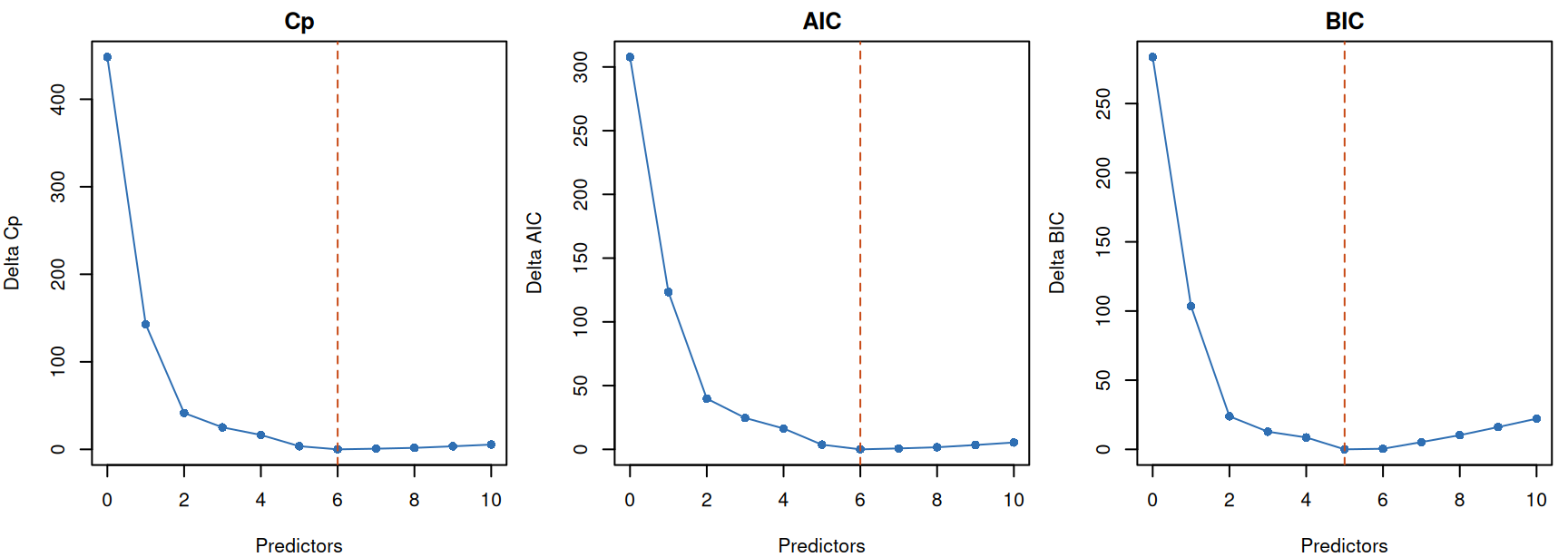
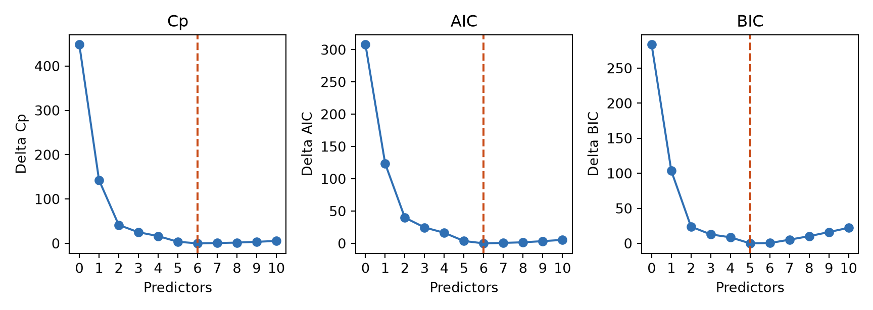
The panels below subtract each criterion’s minimum so that zero marks its preferred size. This normalization changes neither rankings nor selected models.

Show the reproducible code

# Shift each criterion so that its minimum is zero.
cp_gap <- Cp - min(Cp)
aic_gap <- AIC - min(AIC)
bic_gap <- BIC - min(BIC)

# Plot the shifted paths and mark each selected predictor count.
par(mfrow = c(1, 3), mar = c(4, 4, 1.8, 0.7))

plot(
  predictor_count, cp_gap,
  type = "o", pch = 16, col = "#2F6FB3",
  xlab = "Predictors", ylab = "Delta Cp", main = "Cp"
)
abline(v = cp_predictor_count, col = "#C84A16", lty = 2)

plot(
  predictor_count, aic_gap,
  type = "o", pch = 16, col = "#2F6FB3",
  xlab = "Predictors", ylab = "Delta AIC", main = "AIC"
)
abline(v = aic_predictor_count, col = "#C84A16", lty = 2)

plot(
  predictor_count, bic_gap,
  type = "o", pch = 16, col = "#2F6FB3",
  xlab = "Predictors", ylab = "Delta BIC", main = "BIC"
)
abline(v = bic_predictor_count, col = "#C84A16", lty = 2)

Three panels show delta Cp, delta AIC, and delta BIC against number of predictors. Cp and AIC reach zero at six predictors; BIC reaches zero at five. — Best-subset criterion paths by predictor count. Each panel is shifted so its minimum equals zero.

Show the reproducible code

# Shift each criterion so that its minimum is zero.
cp_gap = Cp - Cp.min()
aic_gap = AIC - AIC.min()
bic_gap = BIC - BIC.min()

# Plot the shifted paths and mark each selected predictor count.
fig, axes = plt.subplots(1, 3, figsize=(9, 3.2))

axes[0].plot(predictor_count, cp_gap, "o-", color="#2F6FB3")
axes[0].axvline(cp_predictor_count, color="#C84A16", linestyle="--")
axes[0].set(title="Cp", xlabel="Predictors", ylabel="Delta Cp")

axes[1].plot(predictor_count, aic_gap, "o-", color="#2F6FB3")
axes[1].axvline(aic_predictor_count, color="#C84A16", linestyle="--")
axes[1].set(title="AIC", xlabel="Predictors", ylabel="Delta AIC")

axes[2].plot(predictor_count, bic_gap, "o-", color="#2F6FB3")
axes[2].axvline(bic_predictor_count, color="#C84A16", linestyle="--")
axes[2].set(title="BIC", xlabel="Predictors", ylabel="Delta BIC")

for ax in axes:
    ax.set_xticks(np.arange(0, 11))

fig.tight_layout()
plt.show()

The figure gives more information than the three selected predictor counts. BIC’s best five-predictor model beats its best six-predictor model by only $0.43$ criterion units. AIC’s six-predictor minimum is only about $0.72$ below its seven-predictor value. The software must return one winner, but gaps this small warn us that a slight change in the observations could change the preferred size with little change in the score. That near-tie motivates the stability discussion later in the lecture.

Stepwise selection

With ten predictors, examining all $2^{10}=1{,}024$ subsets is manageable. But the number doubles whenever one predictor is added; with 30 predictors there are more than one billion subsets. Stepwise search is useful because it examines a much smaller collection of models. The price of that speed is that it may miss the overall best model.

Best-subset search asks, “Which candidate has the smallest criterion among all subsets?” Stepwise methods ask a local question: “Which single addition or deletion improves the criterion most from where we are now?”

Forward selection starts from the intercept and adds one predictor at a time.
Backward elimination starts from the full model and removes one predictor at a time.
Bidirectional stepwise permits either move after each step.

The search stops when no allowed one-variable move improves the criterion. Such a stopping point is called a local minimum: it is best among the models one move away, even though a better model may exist elsewhere.

Predict before continuing.

If every one-variable neighbor is worse, has the algorithm proved that every two- or three-variable change is also worse? Keep your answer in mind when we compare the path with exhaustive search.

We focus on one path: forward selection from the intercept-only model using BIC. R’s step() takes the best available addition at each step. Setting k = log(n) gives the BIC penalty; setting k = 2 would use AIC instead.

Show the reproducible code

search_scope <- list(lower = ~1, upper = formula(full_fit))

# Take the best available addition at each step using the BIC penalty.
forward_bic <- step(
  null_fit,
  scope = search_scope,
  direction = "forward",
  k = log(n),
  trace = 0
)

selected_variables <- predictor_names[
  predictor_names %in% names(coef(forward_bic))[-1]
]
forward_bic_rss <- sum(residuals(forward_bic)^2)
forward_bic_parameter_count <- length(coef(forward_bic))
forward_bic_score <- n * log(forward_bic_rss / n) +
  log(n) * forward_bic_parameter_count

formula(forward_bic)

y ~ bmi + s5 + bp + s1 + sex + s2

Forward selection using BIC
criterion	direction	steps	predictors	variables	value
BIC	forward	6	6	sex, bmi, bp, s1, s2, s5	3562.9

Python writes out the same forward search directly. At each step, it evaluates every possible addition, accepts the one with the smallest BIC, and stops when no addition improves the current model.

Show the reproducible code

selected = []
remaining = predictor_names.copy()
current_bic = n * np.log(rss_null / n) + np.log(n)

while remaining:
    # Compare every one-variable extension of the current model.
    candidate_scores = []

    for name in remaining:
        candidate_variables = selected + [name]
        candidate_rss = subset_rss(candidate_variables)
        candidate_parameter_count = len(candidate_variables) + 1
        candidate_bic = (
            n * np.log(candidate_rss / n)
            + np.log(n) * candidate_parameter_count
        )
        candidate_scores.append((candidate_bic, name))

    best_bic, best_name = min(candidate_scores)

    # Stop when even the best available addition does not improve BIC.
    if best_bic >= current_bic:
        break

    # Accept the best addition and continue from the enlarged model.
    selected.append(best_name)
    remaining.remove(best_name)
    current_bic = best_bic

selected_variables = [
    name for name in predictor_names if name in selected
]

selected_variables

['sex', 'bmi', 'bp', 's1', 's2', 's5']

Forward selection using BIC
criterion	direction	steps	predictors	variables	value
BIC	forward	6	6	sex, bmi, bp, s1, s2, s5	3562.90

A worked path: where forward BIC gets stuck

The final selected model is easier to understand if we watch its path develop. Starting from the intercept, forward BIC takes the following moves; “improvement” is the decrease from the previous BIC value.

Step	Model after the move	BIC	Improvement
0	Intercept only	3846.08	not applicable
1	add bmi	3665.88	180.20
2	add s5	3586.33	79.55
3	add bp	3575.25	11.08
4	add s1	3571.08	4.17
5	add sex	3570.29	0.79
6	add s2	3562.90	7.39

The first two moves produce large improvements; later moves change BIC much less. At the six-predictor model, no single allowed addition improves BIC, so forward search stops. Forward search cannot undo the earlier additions of s1 and s2. Exact best-subset search nevertheless finds BIC $3562.47$ for

$\{\text{sex},\text{bmi},\text{bp},\text{s3},\text{s5}\},$

which is $0.43$ lower. Reaching that model requires replacing the pair s1 and s2 by s3. Bidirectional search also stops at the six-predictor model because every single addition or deletion is worse; its best immediate neighbor adds s4 and raises BIC by about $4.81$ . It cannot make the required multi-variable swap without first accepting a worse score. The order in which variables enter only records what helped at each step, given the variables already present. It is not a ranking of causal or scientific importance.

What the algorithms teach us

The exact search and the greedy searches answer related but different questions:

Component	Role	Guarantee
$C_p$ , AIC, or BIC	Assigns a score to any proposed model	Defines what “better” means, subject to its assumptions
Best subset	Searches all relevant subsets	Finds the smallest score among all candidates here
Forward/backward/stepwise	Searches a sequence of one-step neighbors	Stops at the best available one-step move, which may not be best overall

On these data, exact search finds a five-predictor BIC winner containing s3, while the stepwise paths stop at a six-predictor model containing s1 and s2. The difference is caused by the search path, not by BIC itself. A separate issue remains: even the global minimum of a criterion may not be best for the prediction or scientific goal we care about. Keep the limitation of the search method separate from the limitation of the criterion.

The computational trade-off is equally important. Exhaustive search considers $2^p$ subsets. A one-direction greedy path fits at most about $p(p+1)/2$ neighboring models, which is far cheaper for large $p$ , but it makes the result path-dependent.

Stability and honest prediction assessment

The selected subset can change when the data change slightly. This is especially common when predictors are strongly related and can substitute for one another. A selected variable list should therefore be treated as one data-dependent result, not as a permanent ranking of scientific importance.

When cross-validation is used to estimate prediction error, repeat the entire selection procedure inside each training fold:

training fold $\longrightarrow$ select and refit $\longrightarrow$ predict the validation fold.

Selecting variables once using all outcomes and then cross-validating only the final model allows the validation outcomes to influence the variable list indirectly. The resulting error estimate will tend to be too small. Ordinary OLS confidence intervals and p-values also do not account for this model search, so prediction assessment and inference after selection should be treated as different problems.

Check and extend your understanding

Why can training RSS never choose among nested least-squares models by itself?
Why can every subset except one be discarded at each predictor count before comparing $C_p$ , AIC, or BIC?
Does exhaustive search guarantee the best predictive model, or only the candidate with the smallest chosen score?
Change the full-model variance estimate in $C_p$ . Which selected sizes are sensitive to it, and why?
Re-run forward search from a non-null starting model. Does it reach the same local minimum?
Run five-fold cross-validation twice. Inside each training fold, select a best-subset model using BIC in one run and AIC in the other. Compare their mean validation-fold prediction errors.

Key ideas

A criterion assigns a score to a proposed model; a search algorithm decides which proposed models are examined.
Exact best-subset search finds the best value of the chosen criterion over the stated candidates, but it does not guarantee that the criterion matches the scientific goal.
Stepwise search is computationally cheaper because it considers local moves, and those local moves can miss a better model elsewhere.
Prediction error must be assessed for the entire procedure, including search, selection, refitting, and prediction, using outcomes that did not help make those choices.

References and further reading

James, Witten, Hastie, Tibshirani, and Taylor, An Introduction to Statistical Learning, Chapter 6, give an accessible treatment of subset selection, shrinkage, and dimension reduction.
Furnival and Wilson (1974) introduced the leaps-and-bounds ideas behind efficient exact subset search. The official R references are leaps::regsubsets and stats::step.
The official Python references are itertools.combinations for transparent subset enumeration and numpy.linalg.lstsq for stable least-squares fitting.
Derksen and Keselman (1992), Varma and Simon (2006), and Berk et al. (2013) explain, respectively, instability in automated selection, valid resampling after model selection, and the difficulty of inference after selection.