Week 2 Lecture: Training and Testing Errors

On this page

• Overview
• The Problem: Over-fitting
• A Simulation Study
• Key Takeaways
• Theoretical Foundation
• Learning Goals

Overview

In this lecture, we will examine the relationship between training and testing (prediction) errors as model complexity increases. The key insight is the bias-variance trade-off: while training error decreases with more variables, testing error often increases due to over-fitting. We’ll explore this through mathematical derivations and simulation studies.

The Problem: Over-fitting

The central challenge in statistical modeling is that adding more variables always decreases training error (asymptotically reaching zero for perfect fit), but often increases prediction error on fresh data. This is over-fitting.

Consider a simple case: we have \(n\) observations and want to fit a linear regression. When we add more variables, we are using up degrees of freedom. Eventually, the model becomes so flexible that it fits the noise in the training data rather than the true underlying signal. This reduces its ability to generalize to new data.

A Simple Example

Suppose only the first variable is truly useful for predicting the outcome, but we have access to \(p = 20\) variables. What happens if we fit models using 1, 2, 3, …, up to all 20 variables?

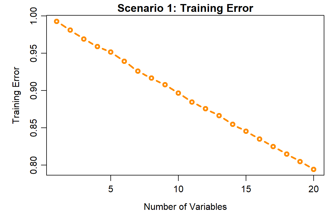
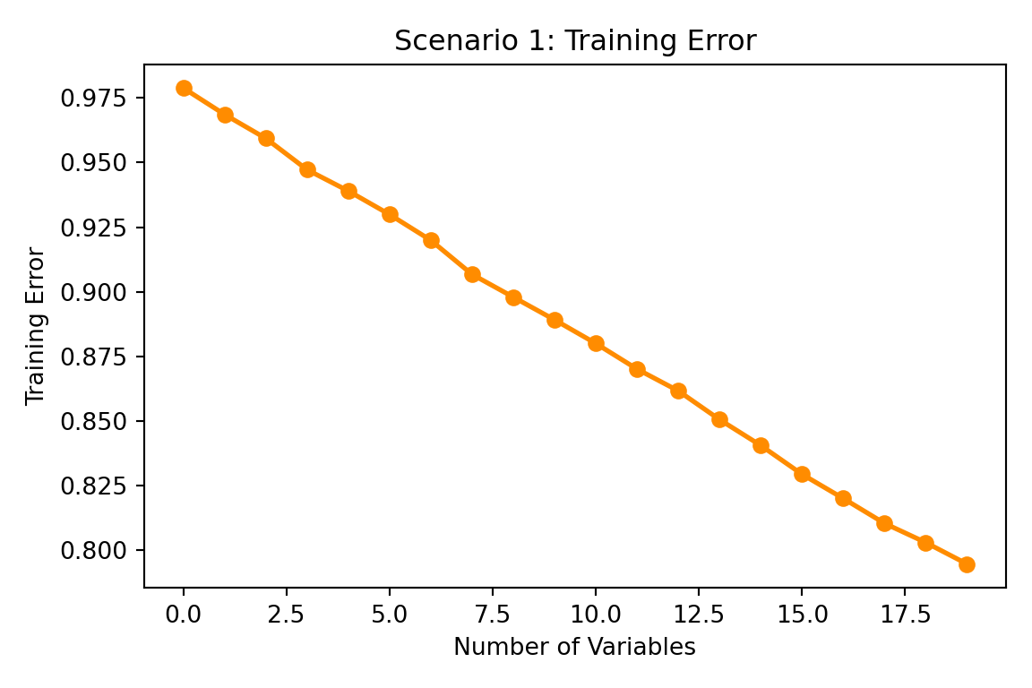
• Training error will continue to decrease (or stay flat).
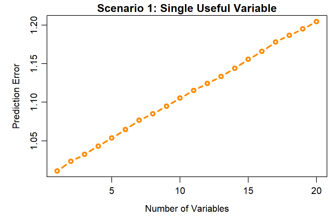
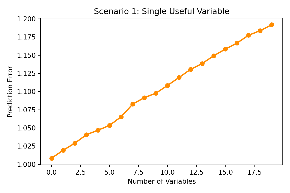
• Prediction error on held-out test data will first decrease, then increase as we add noise variables.

This phenomenon motivates model selection and regularization techniques.

A Simulation Study

The following simulation demonstrates this principle across two scenarios: one where only one variable is useful, and another where variable importance decays gradually.

Scenario 1: Single Useful Variable

We generate data where only the first variable has a signal; all others are pure noise.

\[ Y = 0.3 \cdot X_1 + \varepsilon, \quad \varepsilon \sim N(0, 1) \]

We fit models of increasing size (using variables 1, then 1–2, then 1–3, and so on) and measure both training and prediction error on independent test data. We repeat this 100 times to get a stable estimate.

R

set.seed(1)
n <- 100
p <- 20
nsim <- 100

testerrors <- matrix(NA, nsim, p)
trainerrors <- matrix(NA, nsim, p)

for (i in 1:nsim) {
  x <- matrix(rnorm(n * p), n, p)
  ytrain <- 0.3 * x[, 1] + rnorm(n)
  ytest <- 0.3 * x[, 1] + rnorm(n)
  
  for (j in 1:p) {
    traindata <- data.frame(x = x[, 1:j, drop = FALSE], y = ytrain)
    testdata <- data.frame(x = x[, 1:j, drop = FALSE], y = ytest)
    
    fit <- lm(y ~ ., data = traindata)
    ypred <- predict(fit, testdata)
    
    testerrors[i, j] <- mean((ypred - testdata$y)^2)
    trainerrors[i, j] <- mean((fit$fitted - traindata$y)^2)
  }
}

# Plot prediction error
par(mar = c(4.2, 4.2, 1.4, 0.8), mgp = c(2.3, 0.7, 0))
plot(colMeans(testerrors), type = "b", col = "darkorange", lwd = 3,
     xlab = "Number of Variables", ylab = "Prediction Error",
     main = "Scenario 1: Single Useful Variable")

Python

import numpy as np
import matplotlib.pyplot as plt
from sklearn.linear_model import LinearRegression

np.random.seed(1)
n = 100
p = 20
nsim = 100

testerrors = np.zeros((nsim, p))
trainerrors = np.zeros((nsim, p))

for i in range(nsim):
    x = np.random.normal(size=(n, p))
    ytrain = 0.3 * x[:, 0] + np.random.normal(size=n)
    ytest = 0.3 * x[:, 0] + np.random.normal(size=n)
    
    for j in range(p):
        x_train = x[:, :j+1]
        x_test = x[:, :j+1]
        
        model = LinearRegression()
        model.fit(x_train, ytrain)
        ypred = model.predict(x_test)
        
        testerrors[i, j] = np.mean((ypred - ytest)**2)
        trainerrors[i, j] = np.mean((model.predict(x_train) - ytrain)**2);

plt.figure(figsize=(6, 4))
plt.plot(np.mean(testerrors, axis=0), marker='o', color='darkorange', linewidth=2)
plt.xlabel('Number of Variables')
plt.ylabel('Prediction Error')
plt.title('Scenario 1: Single Useful Variable')
plt.tight_layout()
plt.show()

Comparison: Training Error for Scenario 1

Notice that training error continues to decrease, even though prediction error increases.

R

par(mar = c(4.2, 4.2, 1.4, 0.8), mgp = c(2.3, 0.7, 0))
plot(colMeans(trainerrors), type = "b", col = "darkorange", lwd = 3,
     xlab = "Number of Variables", ylab = "Training Error",
     main = "Scenario 1: Training Error")

Python

plt.figure(figsize=(6, 4))
plt.plot(np.mean(trainerrors, axis=0), marker='o', color='darkorange', linewidth=2)
plt.xlabel('Number of Variables')
plt.ylabel('Training Error')
plt.title('Scenario 1: Training Error')
plt.tight_layout()
plt.show()

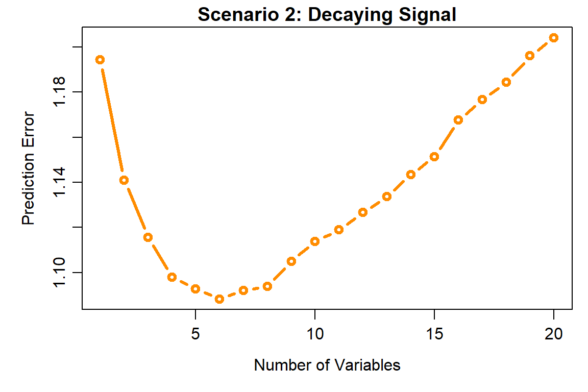
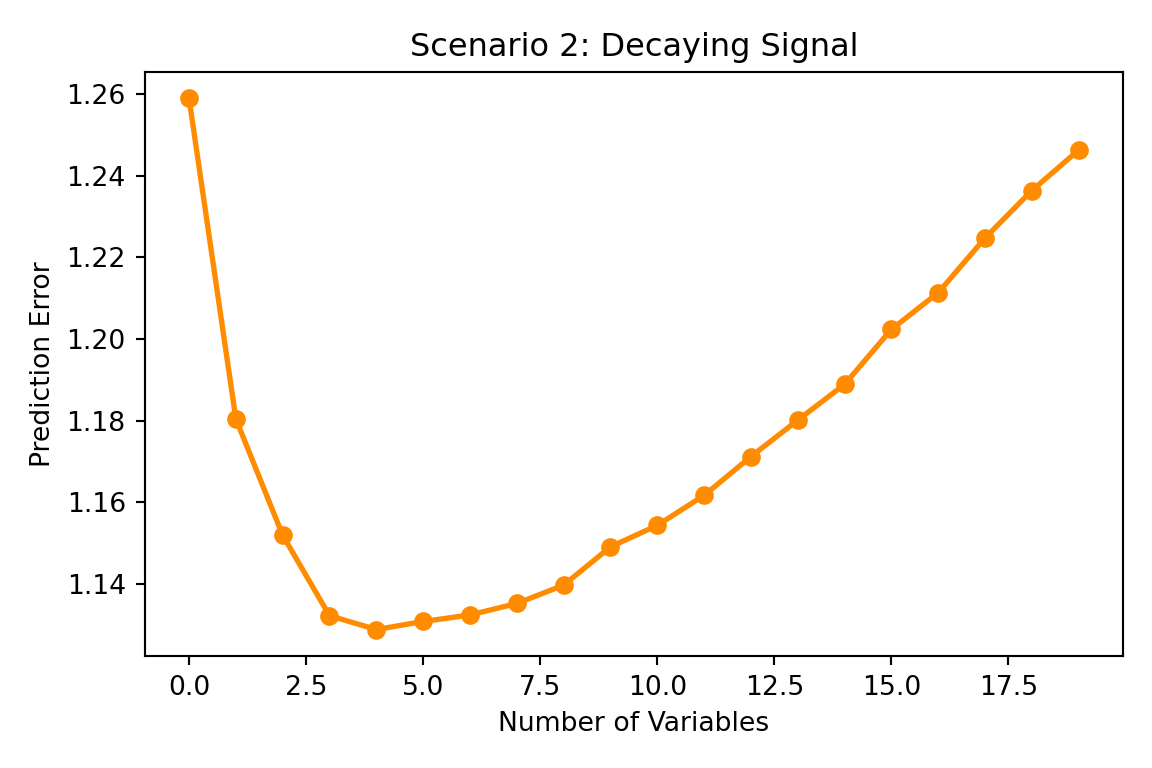
Scenario 2: Decaying Signal

In many real problems, not all variables are useless; instead, their importance decays. Consider:

\[ Y = X^\top \boldsymbol{\beta} + \varepsilon, \quad \beta_j = 0.4^{\sqrt{j}}, \quad j = 1, \ldots, p \]

Here, the first few variables are important, but their effect diminishes with index. Let’s repeat the simulation.

R

testerrors2 <- matrix(NA, nsim, p)
trainerrors2 <- matrix(NA, nsim, p)

for (i in 1:nsim) {
  x <- matrix(rnorm(n * p), n, p)
  beta <- 0.4^sqrt(1:p)
  ytrain <- x %*% beta + rnorm(n)
  ytest <- x %*% beta + rnorm(n)
  
  for (j in 1:p) {
    traindata <- data.frame(x = x[, 1:j, drop = FALSE], y = ytrain)
    testdata <- data.frame(x = x[, 1:j, drop = FALSE], y = ytest)
    
    fit <- lm(y ~ ., data = traindata)
    ypred <- predict(fit, testdata)
    
    testerrors2[i, j] <- mean((ypred - testdata$y)^2)
    trainerrors2[i, j] <- mean((fit$fitted - traindata$y)^2)
  }
}

par(mar = c(4.2, 4.2, 1.4, 0.8), mgp = c(2.3, 0.7, 0))
plot(colMeans(testerrors2), type = "b", col = "darkorange", lwd = 3,
     xlab = "Number of Variables", ylab = "Prediction Error",
     main = "Scenario 2: Decaying Signal")

Python

testerrors2 = np.zeros((nsim, p))
trainerrors2 = np.zeros((nsim, p))

for i in range(nsim):
    x = np.random.normal(size=(n, p))
    beta = 0.4 ** np.sqrt(np.arange(1, p+1))
    ytrain = x @ beta + np.random.normal(size=n)
    ytest = x @ beta + np.random.normal(size=n)
    
    for j in range(p):
        x_train = x[:, :j+1]
        x_test = x[:, :j+1]
        
        model = LinearRegression()
        model.fit(x_train, ytrain)
        ypred = model.predict(x_test)
        
        testerrors2[i, j] = np.mean((ypred - ytest)**2)
        trainerrors2[i, j] = np.mean((model.predict(x_train) - ytrain)**2);

plt.figure(figsize=(6, 4))
plt.plot(np.mean(testerrors2, axis=0), marker='o', color='darkorange', linewidth=2)
plt.xlabel('Number of Variables')
plt.ylabel('Prediction Error')
plt.title('Scenario 2: Decaying Signal')
plt.tight_layout()
plt.show()

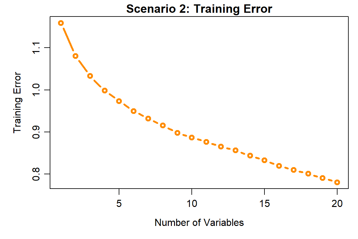
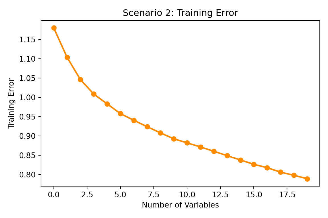
Training Error for Scenario 2

Again, training error steadily decreases, but the benefit of additional variables for prediction is more moderate.

R

par(mar = c(4.2, 4.2, 1.4, 0.8), mgp = c(2.3, 0.7, 0))
plot(colMeans(trainerrors2), type = "b", col = "darkorange", lwd = 3,
     xlab = "Number of Variables", ylab = "Training Error",
     main = "Scenario 2: Training Error")

Python

plt.figure(figsize=(6, 4))
plt.plot(np.mean(trainerrors2, axis=0), marker='o', color='darkorange', linewidth=2)
plt.xlabel('Number of Variables')
plt.ylabel('Training Error')
plt.title('Scenario 2: Training Error')
plt.tight_layout()
plt.show()

Key Takeaways

1. Training error always decreases (or stays the same) as model complexity increases—this is not a reliable guide for choosing model size.

2. Prediction error first decreases then increases—there is an optimal model size that balances fit and complexity.

3. Overfitting occurs when we add too many variables. The model starts fitting noise rather than signal.

4. The optimal model depends on the true signal structure:

   • In Scenario 1 (one useful variable), the best model is very simple.
   • In Scenario 2 (decaying signal), more variables help up to a point.

5. Model selection criteria (AIC, BIC, Cp, cross-validation) are designed to estimate prediction error and find the optimal model size without relying on training error.

Theoretical Foundation

For a correctly specified linear model:

\[ E[\text{Training Error}] = (n-p)\sigma^2 \]

\[ E[\text{Prediction Error}] = (n+p)\sigma^2 \]

The simulation results confirm these formulas when the model is correctly specified. The key insight is that as \(p\) approaches \(n\), training error approaches zero (and becomes unreliable), while prediction error grows due to estimation variance. This is the bias-variance trade-off in action.

Learning Goals

By the end of this section, check if you

1. Understand the difference between training error and prediction error.
2. Explain how overfitting occurs when adding too many variables.
3. Use simulation to verify theoretical predictions about error decomposition.
4. Implement model fitting workflows in both R and Python.