STAT 432
  • Welcome
  • Lectures
    • Overview
    • Week 1: Setup and AI Tools
    • Week 2: Training and Test Error
    • Week 3: Ridge Regression and Optimization
    • Week 4: Lasso and Variable Selection
    • Week 5: K-Nearest Neighbors
    • Week 6: Classification Error and Evaluation
  • Discussion
  • Quizzes
  • Final Project
  • Syllabus
  • Canvas
Skip to main content

Homework 05 Solutions

On this page

  • Before you begin
  • Question 1: Estimate the bias and variance of KNN
  • Question 2: Compare KNN with lasso
  • Question 3: Observed dimension and latent dimension
  • Question 4: Classify handwritten digits
  • Question 5: Create a plot-formatting skill

Before you begin

Each solution repeats the complete question before presenting the reasoning. Questions 1 through 4 include R and Python code; use one language and run its code blocks in order. Question 5 gives an example plot-formatting skill. The code follows the Week 5 lectures, using direct calculations, simple loops, and standard package calls.

The simulation seeds are shown in the code. R and Python use the same models and settings but generate different random observations. Both languages use the same handwritten digit data, row order, and tie rules. The digit data are loaded directly from ElemStatLearn in R and from the supplied course copies in Python, as requested in Question 4.

Download the materials

  • Download solutions-05.qmd
  • Download homework-05.qmd
  • Download combined ZIP file

The ZIP file contains the two editable QMD files and the handwritten digit data for Python in Question 4. The solution code generates all simulation results and figures.

Question 1: Estimate the bias and variance of KNN

Original question

In our previous homework, we used repeated simulations to study the behavior of linear regression estimators. We will now use the same idea for KNN. Consider the regression model

Yi=f(𝑿i)+Ο΅i,f(𝒙)=0.5x1+sin⁑(x2)βˆ’0.3x32, Y_i=f(\mathbf X_i)+\epsilon_i, \qquad f(\mathbf x)=0.5x_1+\sin(x_2)-0.3x_3^2,

where the three covariates are independent standard normal variables and Ο΅iβˆΌπ’©(0,0.12)\epsilon_i\sim\mathcal N(0,0.1^2) independently of the covariates and other observations. Generate n=400n=400 training observations. Our goal is to estimate the mean response at

𝒙0=(0.5,0.7,1)𝖳. \mathbf x_0=(0.5,0.7,1)^{\mathsf T}.

Use Euclidean distance and consider k=1,3,5,…,29k=1,3,5,\ldots,29.

  1. Calculate f(𝒙0)f(\mathbf x_0). Generate one training dataset and obtain the KNN prediction at 𝒙0\mathbf x_0 for each value of kk.

  2. Independently repeat the generation of the training covariates and responses 200 times. Within each repetition, use the same training data for every value of kk. Store the predictions in a matrix with 200 rows and one column for each value of kk. Use this matrix to estimate the bias, variance, and mean squared error of the estimated mean response. Use divisor 200 when calculating the empirical variance, and verify numerically that

mean squared error=squared bias+variance. \text{mean squared error} =\text{squared bias}+\text{variance}.

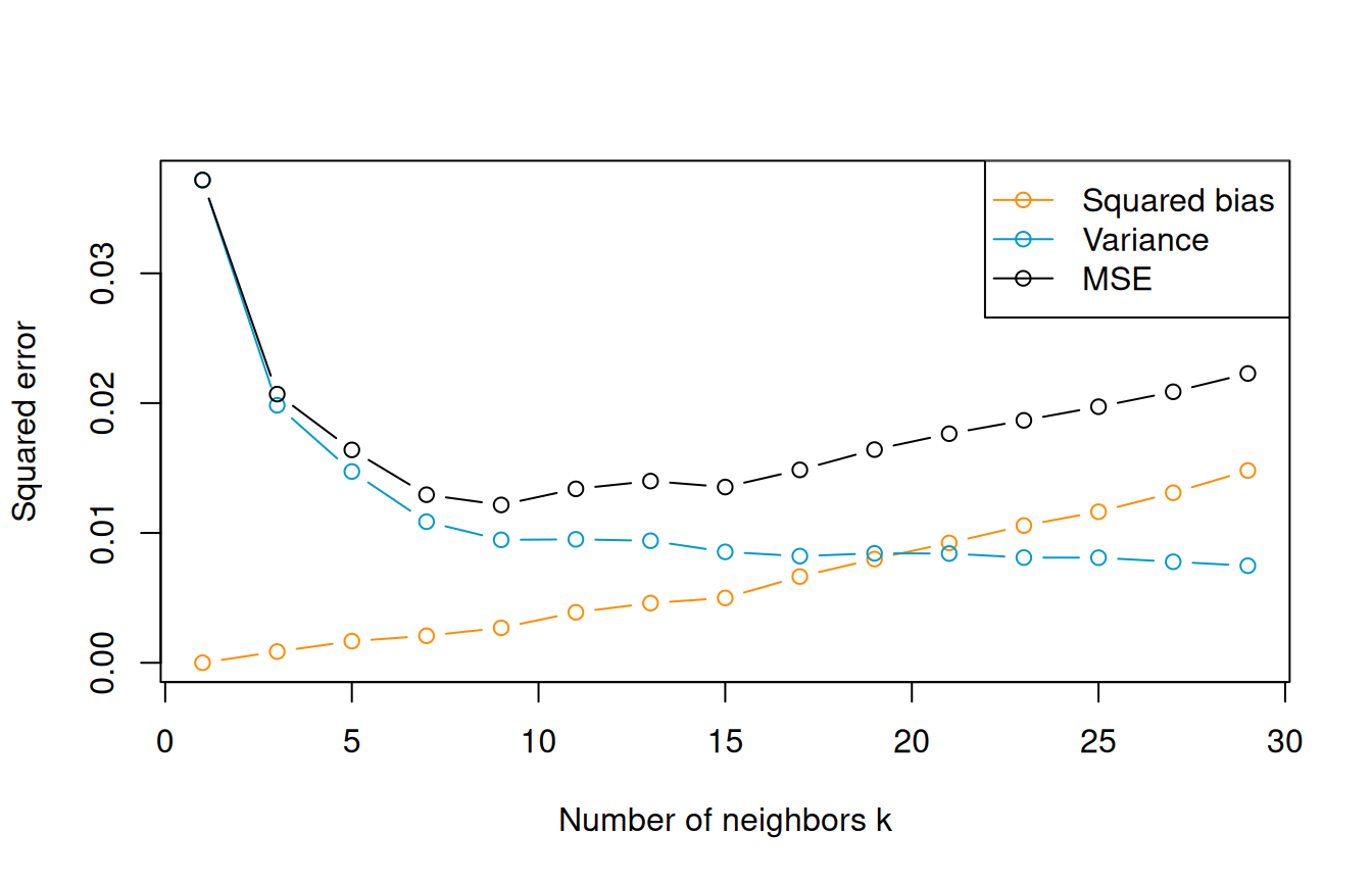
Plot squared bias, variance, and mean squared error against kk in one figure. Explain the pattern and compare it with the bias-variance trade-off for ridge regression or lasso.

Solution

a. The target is the mean response, whose true value is

f(𝒙0)=0.5(0.5)+sin⁑(0.7)βˆ’0.3(1)2β‰ˆ0.594218. f(\mathbf x_0)=0.5(0.5)+\sin(0.7)-0.3(1)^2 \approx 0.594218.

We first generate one training dataset and average the responses of the nearest kk observations for each choice of kk.

  • R
  • Python
Show the solution code
library(FNN)
set.seed(43251)
n = 400
p = 3
k_values = seq(1, 29, 2)
x0 = matrix(c(0.5, 0.7, 1), nrow = 1)
f0 = 0.5*x0[1, 1] + sin(x0[1, 2]) - 0.3*x0[1, 3]^2

X = matrix(rnorm(n*p), nrow = n, ncol = p)
y = 0.5*X[, 1] + sin(X[, 2]) - 0.3*X[, 3]^2 + rnorm(n, sd = 0.1)
pred = numeric(length(k_values))
for (m in seq_along(k_values)) {
  k = k_values[m]
  knn.fit = knn.reg(train = X, test = x0, y = y,
                    k = k, algorithm = "brute")
  pred[m] = knn.fit$pred
}
data.frame(k = k_values, prediction = pred, truth = f0)
    k prediction     truth
1   1  0.7888302 0.5942177
2   3  0.6621674 0.5942177
3   5  0.6642853 0.5942177
4   7  0.6100117 0.5942177
5   9  0.6318671 0.5942177
6  11  0.4925114 0.5942177
7  13  0.5222989 0.5942177
8  15  0.5810203 0.5942177
9  17  0.5738171 0.5942177
10 19  0.5751479 0.5942177
11 21  0.5800517 0.5942177
12 23  0.5519177 0.5942177
13 25  0.5214556 0.5942177
14 27  0.4952957 0.5942177
15 29  0.4972667 0.5942177
Show the solution code
import numpy as np
import pandas as pd
import matplotlib.pyplot as plt
from sklearn.neighbors import KNeighborsRegressor

np.random.seed(43251)
n = 400
p = 3
k_values = np.arange(1, 30, 2)
x0 = np.array([[0.5, 0.7, 1]])
f0 = 0.5*x0[0, 0] + np.sin(x0[0, 1]) - 0.3*x0[0, 2]**2

X = np.random.normal(size=(n, p))
y = (0.5*X[:, 0] + np.sin(X[:, 1]) - 0.3*X[:, 2]**2
     + np.random.normal(0, 0.1, n))
pred = np.zeros(len(k_values))
for m, k in enumerate(k_values):
    knn_fit = KNeighborsRegressor(n_neighbors=int(k), weights="uniform",
                                  algorithm="brute")
    knn_fit.fit(X, y)
    pred[m] = knn_fit.predict(x0)[0]
print(pd.DataFrame({"k": k_values, "prediction": pred, "truth": f0}))
     k  prediction     truth
0    1    0.847540  0.594218
1    3    0.570740  0.594218
2    5    0.642444  0.594218
3    7    0.614333  0.594218
4    9    0.641423  0.594218
5   11    0.576739  0.594218
6   13    0.556318  0.594218
7   15    0.551736  0.594218
8   17    0.578973  0.594218
9   19    0.611623  0.594218
10  21    0.529554  0.594218
11  23    0.515161  0.594218
12  25    0.557332  0.594218
13  27    0.518179  0.594218
14  29    0.538406  0.594218

b. Each column of the prediction matrix contains 200 estimates of the same target. Its mean minus f(𝒙0)f(\mathbf x_0) estimates bias; its variance, calculated with divisor 200, estimates sampling variance. Averaging the squared differences from f(𝒙0)f(\mathbf x_0) estimates MSE. Using the same divisor makes the empirical decomposition an exact identity, apart from rounding.

  • R
  • Python
Show the solution code
nsim = 200
pred = matrix(NA, nrow = nsim, ncol = length(k_values))
for (l in 1:nsim) {
  X = matrix(rnorm(n*p), nrow = n, ncol = p)
  y = 0.5*X[, 1] + sin(X[, 2]) - 0.3*X[, 3]^2 + rnorm(n, sd = 0.1)
  for (m in seq_along(k_values)) {
    k = k_values[m]
    knn.fit = knn.reg(train = X, test = x0, y = y,
                      k = k, algorithm = "brute")
    pred[l, m] = knn.fit$pred
  }
}
bias = colMeans(pred) - f0
variance = colMeans(sweep(pred, 2, colMeans(pred), "-")^2)
mse = colMeans((pred - f0)^2)
data.frame(k = k_values, bias = bias, variance = variance, MSE = mse)
    k         bias    variance        MSE
1   1 -0.001248923 0.037181204 0.03718276
2   3 -0.029361680 0.019831580 0.02069369
3   5 -0.040815728 0.014731018 0.01639694
4   7 -0.045589732 0.010865566 0.01294399
5   9 -0.051867114 0.009467440 0.01215764
6  11 -0.062360901 0.009506180 0.01339506
7  13 -0.067797856 0.009397702 0.01399425
8  15 -0.070662763 0.008542311 0.01353554
9  17 -0.081499864 0.008213727 0.01485595
10 19 -0.089385641 0.008429774 0.01641957
11 21 -0.096080776 0.008413451 0.01764497
12 23 -0.102803643 0.008103017 0.01867161
13 25 -0.107847900 0.008091147 0.01972232
14 27 -0.114428351 0.007777947 0.02087180
15 29 -0.121688194 0.007474576 0.02228259
Show the solution code
max(abs(mse - bias^2 - variance))
[1] 6.938894e-18
Show the solution code
matplot(k_values, cbind(bias^2, variance, mse), type = "b", pch = 1,
        lty = 1, col = c("darkorange", "deepskyblue3", "black"),
        xlab = "Number of neighbors k", ylab = "Squared error",
        ylim = c(0, max(mse)))
legend("topright", c("Squared bias", "Variance", "MSE"),
       col = c("darkorange", "deepskyblue3", "black"), lty = 1, pch = 1)

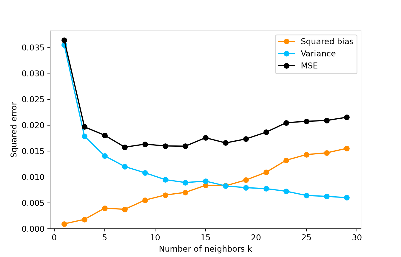
Squared bias, variance, and mean squared error at the fixed target as the number of neighbors increases.

Show the solution code
nsim = 200
pred = np.full((nsim, len(k_values)), np.nan)
for l in range(nsim):
    X = np.random.normal(size=(n, p))
    y = (0.5*X[:, 0] + np.sin(X[:, 1]) - 0.3*X[:, 2]**2
         + np.random.normal(0, 0.1, n))
    for m, k in enumerate(k_values):
        knn_fit = KNeighborsRegressor(n_neighbors=int(k), weights="uniform",
                                      algorithm="brute")
        knn_fit.fit(X, y)
        pred[l, m] = knn_fit.predict(x0)[0]

bias = pred.mean(axis=0) - f0
variance = pred.var(axis=0, ddof=0)
mse = ((pred - f0)**2).mean(axis=0)
print(pd.DataFrame({"k": k_values, "bias": bias,
                    "variance": variance, "MSE": mse}))
     k      bias  variance       MSE
0    1 -0.030696  0.035483  0.036426
1    3 -0.042477  0.017863  0.019667
2    5 -0.063010  0.014078  0.018048
3    7 -0.061247  0.012000  0.015751
4    9 -0.074360  0.010798  0.016327
5   11 -0.080647  0.009484  0.015988
6   13 -0.083765  0.008917  0.015934
7   15 -0.091509  0.009190  0.017564
8   17 -0.091101  0.008264  0.016563
9   19 -0.096967  0.007931  0.017334
10  21 -0.104375  0.007739  0.018633
11  23 -0.115020  0.007236  0.020465
12  25 -0.119638  0.006421  0.020735
13  27 -0.121039  0.006248  0.020899
14  29 -0.124566  0.006007  0.021524
Show the solution code
print("Largest decomposition difference:", np.max(np.abs(mse - bias**2 - variance)))
Largest decomposition difference: 1.1188966420050406e-16
Show the solution code
plt.figure(figsize=(7, 4.5))
plt.plot(k_values, bias**2, "o-", color="darkorange", label="Squared bias")
plt.plot(k_values, variance, "o-", color="deepskyblue", label="Variance")
plt.plot(k_values, mse, "o-", color="black", label="MSE")
plt.xlabel("Number of neighbors k")
plt.ylabel("Squared error")
plt.ylim(bottom=0)
plt.legend()
plt.show()

Squared bias, variance, and mean squared error at the fixed target as the number of neighbors increases.

Larger kk averages more responses, reducing variability, but it also includes observations farther from the target. Their mean responses can differ more from f(𝒙0)f(\mathbf x_0), introducing bias. Here an intermediate neighborhood gives a lower MSE than either very few or many neighbors. Small irregularities in the curves are expected with 200 repetitions; monotonic changes in each component are not guaranteed.

Increasing kk plays a similar smoothing role to increasing the penalty in ridge regression or lasso: predictions become less flexible, with a trade-off between bias and variance. KNN changes which local responses are averaged; ridge and lasso shrink fitted coefficients. In this experiment both the training locations and their responses change across repetitions, so the variance includes changing neighborhoods as well as response noise. It is therefore not simply 0.12/k0.1^2/k, which describes the conditional noise variance when the neighbor locations are fixed.

Question 2: Compare KNN with lasso

Original question

Use the response model from Question 1, including the noise standard deviation 0.10.1, but generate p=30p=30 covariates. The response still depends only on the first three. Consider these two settings:

  • Setting 1: all 30 covariates are independent standard normal variables.

  • Setting 2: the covariates have a multivariate normal distribution with mean zero and covariance matrix 𝚺\boldsymbol\Sigma, where

    Σjj=1,Σjl=0.8for j≠l. \Sigma_{jj}=1, \qquad \Sigma_{jl}=0.8\quad\text{for }j\ne l.

In each setting, generate 400 training observations and 1,000 independent test observations. Fit 5NN using Euclidean distance on the supplied covariate scale. All covariates already have population variance one.

For lasso, use a linear model containing the 30 covariates and a separately fitted, unpenalized intercept. Follow the Week 4 objective,

LΞ»(𝜷)=12nβˆ₯π’šΜƒβˆ’π‘Ώπœ·βˆ₯22+Ξ»β€–πœ·β€–1, L_\lambda(\boldsymbol\beta) =\frac{1}{2n}\left\lVert \widetilde{\mathbf y}-\mathbf X\boldsymbol\beta \right\rVert_2^2 +\lambda\lVert\boldsymbol\beta\rVert_1,

where π‘Ώβˆˆβ„nΓ—30\mathbf X\in\mathbb R^{n\times30} contains the centered and standardized covariates and π’šΜƒ\widetilde{\mathbf y} is the centered training response. Select the penalty by ten-fold cross-validation over 41 logarithmically spaced values from 10βˆ’410^{-4} to 11. Estimate all means and scales using only the training portion of each fold, with divisor equal to that portion’s sample size. After selecting the penalty, refit on all training observations and apply the fitted transformations unchanged to the test observations. Do not add nonlinear terms to the lasso model.

  1. Fit both methods in each setting. Use the same training and test data for the two methods within a setting. Report their test MSE values in one table, together with the selected lasso penalty and the number of nonzero lasso slopes. You only need to generate one dataset for each setting; repeated simulations are not required.

  2. Compare the results between the two settings. Explain how correlation can change the usefulness of Euclidean neighborhoods, and why lasso does not use all covariates in the same way as KNN.

  3. The response model contains sin⁑(X2)\sin(X_2) and X32X_3^2, but the lasso fit uses only linear terms. Explain how this difference affects the comparison. Would the results justify a general claim that correlation always helps KNN, or that one method is always better? Explain why.

Solution

a. We compare the two methods on the same observations within each setting. KNN uses all 30 covariates when finding neighbors. Lasso can set slopes to zero, but it is restricted to a linear prediction rule. The following code selects the lasso penalty using training data only.

  • R
  • Python
Show the solution code
library(FNN)
library(glmnet)
set.seed(43252)

n <- 400
p <- 30
lambda <- 10^seq(0, -4, length.out = 41)
results <- data.frame(
  Setting = c("Independent", "Correlated"),
  KNN_MSE = NA_real_, Lasso_MSE = NA_real_,
  Lambda = NA_real_, Nonzero = NA_integer_
)

for (l in 1:2) {
  Sigma <- diag(p)
  if (l == 2) Sigma <- 0.8 + 0.2 * diag(p)

  X <- matrix(rnorm((n + 1000) * p), ncol = p) %*% chol(Sigma)
  y <- 0.5 * X[, 1] + sin(X[, 2]) - 0.3 * X[, 3]^2 +
    rnorm(n + 1000, sd = 0.1)
  test.X <- X[(n + 1):(n + 1000), ]
  test.y <- y[(n + 1):(n + 1000)]
  X <- X[1:n, ]
  y <- y[1:n]

  knn.fit <- knn.reg(X, test.X, y, k = 5, algorithm = "brute")
  results$KNN_MSE[l] <- mean((test.y - knn.fit$pred)^2)

  # Estimate means and scales separately in each training fold.
  fold <- sample(rep(1:10, each = n / 10))
  cv.mse <- matrix(NA_real_, nrow = 10, ncol = length(lambda))
  for (m in 1:10) {
    X.mean <- colMeans(X[fold != m, ])
    X.fit <- sweep(X[fold != m, ], 2, X.mean, "-")
    X.sd <- sqrt(colMeans(X.fit^2))
    X.fit <- sweep(X.fit, 2, X.sd, "/")
    X.valid <- sweep(X[fold == m, ], 2, X.mean, "-")
    X.valid <- sweep(X.valid, 2, X.sd, "/")
    y.mean <- mean(y[fold != m])

    lasso.fit <- glmnet(
      X.fit, y[fold != m] - y.mean, alpha = 1, lambda = lambda,
      intercept = FALSE, standardize = FALSE
    )
    y.hat <- predict(lasso.fit, newx = X.valid, s = lambda) + y.mean
    cv.mse[m, ] <- colMeans((y[fold == m] - y.hat)^2)
  }
  lambda.min <- lambda[which.min(colMeans(cv.mse))]

  # Refit using all training observations and keep these transformations.
  X.mean <- colMeans(X)
  X.fit <- sweep(X, 2, X.mean, "-")
  X.sd <- sqrt(colMeans(X.fit^2))
  X.fit <- sweep(X.fit, 2, X.sd, "/")
  test.X.fit <- sweep(test.X, 2, X.mean, "-")
  test.X.fit <- sweep(test.X.fit, 2, X.sd, "/")
  y.mean <- mean(y)
  lasso.fit <- glmnet(
    X.fit, y - y.mean, alpha = 1, lambda = lambda,
    intercept = FALSE, standardize = FALSE
  )
  test.pred <- as.vector(
    predict(lasso.fit, newx = test.X.fit, s = lambda.min)
  ) + y.mean

  results$Lasso_MSE[l] <- mean((test.y - test.pred)^2)
  results$Lambda[l] <- lambda.min
  results$Nonzero[l] <- sum(coef(lasso.fit, s = lambda.min)[-1, 1] != 0)
}
knitr::kable(results, digits = 4)
Setting KNN_MSE Lasso_MSE Lambda Nonzero
Independent 0.5565 0.2602 0.0251 11
Correlated 0.1609 0.2259 0.0100 16
Show the solution code
import numpy as np
import pandas as pd
from sklearn.neighbors import KNeighborsRegressor
from sklearn.linear_model import Lasso

np.random.seed(43252)
n = 400
p = 30
lambda_grid = np.logspace(0, -4, 41)
results = pd.DataFrame({
    "Setting": ["Independent", "Correlated"],
    "KNN_MSE": np.nan, "Lasso_MSE": np.nan,
    "Lambda": np.nan, "Nonzero": 0
})

for l in range(2):
    Sigma = np.eye(p)
    if l == 1:
        Sigma = 0.8 + 0.2 * np.eye(p)

    X = np.random.normal(size=(n + 1000, p)) @ np.linalg.cholesky(Sigma).T
    y = (0.5 * X[:, 0] + np.sin(X[:, 1]) - 0.3 * X[:, 2]**2
         + np.random.normal(scale=0.1, size=n + 1000))
    test_X = X[n:, :]
    test_y = y[n:]
    X = X[:n, :]
    y = y[:n]

    knn_fit = KNeighborsRegressor(n_neighbors=5, weights="uniform",
                                  algorithm="brute")
    knn_fit.fit(X, y)
    results.loc[l, "KNN_MSE"] = np.mean((test_y - knn_fit.predict(test_X))**2)

    # Estimate means and scales separately in each training fold.
    fold = np.random.permutation(np.repeat(np.arange(10), n // 10))
    cv_mse = np.zeros((10, len(lambda_grid)))
    for m in range(10):
        X_mean = X[fold != m, :].mean(axis=0)
        X_sd = X[fold != m, :].std(axis=0, ddof=0)
        X_fit = (X[fold != m, :] - X_mean) / X_sd
        X_valid = (X[fold == m, :] - X_mean) / X_sd
        y_mean = y[fold != m].mean()

        for h in range(len(lambda_grid)):
            lasso_fit = Lasso(alpha=lambda_grid[h], fit_intercept=False,
                              tol=1e-8, max_iter=100000)
            lasso_fit.fit(X_fit, y[fold != m] - y_mean)
            y_hat = lasso_fit.predict(X_valid) + y_mean
            cv_mse[m, h] = np.mean((y[fold == m] - y_hat)**2)
    lambda_min = lambda_grid[np.argmin(cv_mse.mean(axis=0))]

    # Refit using all training observations and keep these transformations.
    X_mean = X.mean(axis=0)
    X_sd = X.std(axis=0, ddof=0)
    X_fit = (X - X_mean) / X_sd
    test_X_fit = (test_X - X_mean) / X_sd
    y_mean = y.mean()
    lasso_fit = Lasso(alpha=lambda_min, fit_intercept=False,
                      tol=1e-8, max_iter=100000)
    lasso_fit.fit(X_fit, y - y_mean)
    test_pred = lasso_fit.predict(test_X_fit) + y_mean

    results.loc[l, "Lasso_MSE"] = np.mean((test_y - test_pred)**2)
    results.loc[l, "Lambda"] = lambda_min
    results.loc[l, "Nonzero"] = np.count_nonzero(lasso_fit.coef_)
print(results.round(4).to_string(index=False))
    Setting  KNN_MSE  Lasso_MSE  Lambda  Nonzero
Independent   0.5640     0.2344  0.0316        9
 Correlated   0.1729     0.2421  0.0316        2

The scales use divisor equal to the number of observations being fitted. Centering the response and adding its mean back gives an unpenalized intercept. Here glmnet’s lambda and scikit-learn’s alpha both use the penalty in the stated 1/(2n)1/(2n) objective; glmnet’s alpha = 1 requests lasso. R and Python generate different observations, so their numerical results need not match.

b. In these realizations, lasso has the smaller test MSE with independent covariates, whereas KNN has the smaller test MSE with correlated covariates. With independent covariates, many coordinates that do not affect the response contribute to Euclidean distance. The nearest observations in 30-dimensional Euclidean distance need not be the nearest in the three relevant coordinates.

With strong positive correlation, the covariates share substantial variation. Euclidean neighborhoods can then be more informative about the response-relevant coordinates. Lasso treats covariates differently: it estimates a separate slope for each and can set some slopes to zero. In the correlated setting, a covariate outside the first three can also act as a proxy for a relevant covariate, and several correlated covariates can compete in the fitted model.

c. Lasso uses X2X_2 and X3X_3 as linear terms, so it cannot reproduce sin⁑(X2)\sin(X_2) or the quadratic contribution βˆ’0.3X32-0.3X_3^2. Its intercept can account for the average quadratic contribution, but not its variation across observations. KNN does not impose a linear form, although its accuracy depends on whether it finds informative neighbors. The comparison therefore reflects both neighborhood quality and the restrictions of the fitted lasso model. Two single datasets do not show that correlation always helps KNN or that either method is universally better.

Question 3: Observed dimension and latent dimension

Original question

The lecture’s handwritten digit example shows that KNN can work with many measured covariates. We will use a simulation to investigate why the structure of those covariates matters.

Let p=100p=100 be the number of observed covariates and let mm be the number of latent variables. For each observation, generate

𝑿i=𝑨𝒁i+𝜼i,Yi=Zi1+Zi2+Ο΅i, \mathbf X_i=\mathbf A\mathbf Z_i+\boldsymbol\eta_i, \qquad Y_i=Z_{i1}+Z_{i2}+\epsilon_i,

where π‘¨βˆˆβ„100Γ—m\mathbf A\in\mathbb R^{100\times m} has independent entries from Uniform[βˆ’2,2][-2,2]. The entries of 𝒁iβˆˆβ„m\mathbf Z_i\in\mathbb R^m and 𝜼iβˆˆβ„100\boldsymbol\eta_i\in\mathbb R^{100}, and the scalar Ο΅i\epsilon_i, are independent standard normal variables, also independent of 𝑨\mathbf A. Generate 𝑨\mathbf A once and use it for all training and test observations in that dataset.

Compare m=3m=3 and m=30m=30. In each setting, generate 200 training observations and 200 independent test observations. Fit KNN using only the 100 observed covariates in 𝑿\mathbf X, with Euclidean distance on their generated scale. The latent variables in 𝒁\mathbf Z are used to generate the data but are not available to the fitted model. Consider k=2,10,18,…,82k=2,10,18,\ldots,82.

  1. Generate one dataset for each value of mm. Fit KNN for every value of kk and calculate test MSE. Within a setting, use the same training and test observations for all values of kk.

  2. Repeat the complete experiment 50 times, generating a new 𝑨\mathbf A and new observations in each repetition. Plot average test MSE against kk, with one curve for each value of mm. These curves compare the specified choices of kk in a controlled simulation; they are not a cross-validation procedure for selecting a final model.

  3. Both settings have 100 observed covariates, and the response depends on only two latent variables. Explain why their KNN performance can still differ. What role does the noise 𝜼i\boldsymbol\eta_i play, and why are the observed data not confined exactly to an mm-dimensional linear space?

Solution

a. The observed dimension is 100 in both settings. We generate the training and test observations using the same matrix 𝑨\mathbf A, then use only 𝑿\mathbf X to fit KNN.

  • R
  • Python
Show the solution code
library(FNN)
set.seed(43254)
p = 100
m_values = c(3, 30)
k_values = seq(2, 82, 8)
test_mse = matrix(NA, nrow = length(k_values), ncol = 2)

for (m in m_values) {
  A = matrix(runif(p*m, -2, 2), nrow = p, ncol = m)
  Z = matrix(rnorm(400*m), nrow = 400, ncol = m)
  X = Z %*% t(A) + matrix(rnorm(400*p), nrow = 400, ncol = p)
  y = Z[, 1] + Z[, 2] + rnorm(400)
  for (k in k_values) {
    knn.fit = knn.reg(train = X[1:200, ], test = X[201:400, ],
                      y = y[1:200], k = k, algorithm = "brute")
    test_mse[match(k, k_values), match(m, m_values)] =
      mean((y[201:400] - knn.fit$pred)^2)
  }
}
data.frame(k = k_values, m3 = test_mse[, 1], m30 = test_mse[, 2])
    k       m3      m30
1   2 1.449265 3.457456
2  10 1.253345 2.583372
3  18 1.292923 2.533071
4  26 1.379955 2.524038
5  34 1.448416 2.512187
6  42 1.505892 2.560783
7  50 1.590057 2.562911
8  58 1.660186 2.593970
9  66 1.739597 2.607162
10 74 1.816963 2.651181
11 82 1.871802 2.672724
Show the solution code
import numpy as np
import pandas as pd
import matplotlib.pyplot as plt
from sklearn.neighbors import KNeighborsRegressor

np.random.seed(43254)
p = 100
m_values = [3, 30]
k_values = np.arange(2, 83, 8)
test_mse = np.full((len(k_values), 2), np.nan)

for s, m in enumerate(m_values):
    A = np.random.uniform(-2, 2, size=(p, m))
    Z = np.random.normal(size=(400, m))
    X = Z @ A.T + np.random.normal(size=(400, p))
    y = Z[:, 0] + Z[:, 1] + np.random.normal(size=400)
    for l, k in enumerate(k_values):
        knn_fit = KNeighborsRegressor(n_neighbors=int(k), weights="uniform",
                                      algorithm="brute")
        knn_fit.fit(X[:200], y[:200])
        test_mse[l, s] = np.mean((y[200:] - knn_fit.predict(X[200:]))**2)
print(pd.DataFrame({"k": k_values, "m=3": test_mse[:, 0],
                    "m=30": test_mse[:, 1]}))
     k       m=3      m=30
0    2  1.497394  2.533618
1   10  1.139600  2.097571
2   18  1.211048  1.965676
3   26  1.285690  1.926529
4   34  1.345035  1.958095
5   42  1.405158  2.011077
6   50  1.477098  2.058123
7   58  1.551437  2.098877
8   66  1.609162  2.117440
9   74  1.672598  2.148940
10  82  1.732583  2.179772

b. The following loop repeats the entire experiment, including generation of 𝑨\mathbf A. The result array stores repetitions, choices of kk, and the two latent dimensions along its three axes.

  • R
  • Python
Show the solution code
nsim = 50
test_mse = array(NA, dim = c(nsim, length(k_values), 2))
for (l in 1:nsim) {
  for (m in m_values) {
    A = matrix(runif(p*m, -2, 2), nrow = p, ncol = m)
    Z = matrix(rnorm(400*m), nrow = 400, ncol = m)
    X = Z %*% t(A) + matrix(rnorm(400*p), nrow = 400, ncol = p)
    y = Z[, 1] + Z[, 2] + rnorm(400)
    for (k in k_values) {
      knn.fit = knn.reg(train = X[1:200, ], test = X[201:400, ],
                        y = y[1:200], k = k, algorithm = "brute")
      test_mse[l, match(k, k_values), match(m, m_values)] =
        mean((y[201:400] - knn.fit$pred)^2)
    }
  }
}
mean_mse = apply(test_mse, c(2, 3), mean)
data.frame(k = k_values, m3 = mean_mse[, 1], m30 = mean_mse[, 2])
    k       m3      m30
1   2 1.634822 3.062662
2  10 1.288062 2.349524
3  18 1.321139 2.345840
4  26 1.372628 2.378219
5  34 1.437850 2.412709
6  42 1.496497 2.455664
7  50 1.554715 2.492101
8  58 1.615062 2.527212
9  66 1.673644 2.556039
10 74 1.736733 2.589309
11 82 1.800274 2.618853
Show the solution code
matplot(k_values, mean_mse, type = "b", pch = c(1, 2), lty = 1,
        col = c("deepskyblue3", "darkorange"),
        xlab = "Number of neighbors k", ylab = "Average test MSE")
legend("topright", c("m = 3", "m = 30"),
       col = c("deepskyblue3", "darkorange"), lty = 1, pch = c(1, 2))

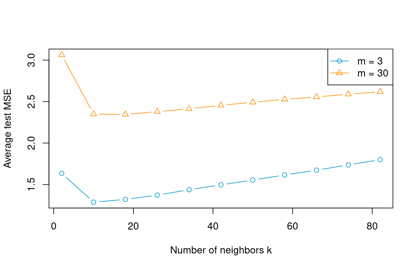
Average test MSE across 50 repetitions for latent dimensions 3 and 30, both observed through 100 covariates.

Show the solution code
nsim = 50
test_mse = np.full((nsim, len(k_values), 2), np.nan)
for l in range(nsim):
    for s, m in enumerate(m_values):
        A = np.random.uniform(-2, 2, size=(p, m))
        Z = np.random.normal(size=(400, m))
        X = Z @ A.T + np.random.normal(size=(400, p))
        y = Z[:, 0] + Z[:, 1] + np.random.normal(size=400)
        for h, k in enumerate(k_values):
            knn_fit = KNeighborsRegressor(n_neighbors=int(k), weights="uniform",
                                          algorithm="brute")
            knn_fit.fit(X[:200], y[:200])
            test_mse[l, h, s] = np.mean((y[200:] - knn_fit.predict(X[200:]))**2)

mean_mse = test_mse.mean(axis=0)
print(pd.DataFrame({"k": k_values, "m=3": mean_mse[:, 0],
                    "m=30": mean_mse[:, 1]}))
     k       m=3      m=30
0    2  1.690342  3.071050
1   10  1.303540  2.312968
2   18  1.330768  2.289224
3   26  1.380082  2.311756
4   34  1.432114  2.333897
5   42  1.488269  2.368583
6   50  1.544620  2.398708
7   58  1.600520  2.425605
8   66  1.654332  2.456120
9   74  1.711747  2.483537
10  82  1.773539  2.511958
Show the solution code
plt.figure(figsize=(7, 4.5))
plt.plot(k_values, mean_mse[:, 0], "o-", color="deepskyblue", label="m = 3")
plt.plot(k_values, mean_mse[:, 1], "^-", color="darkorange", label="m = 30")
plt.xlabel("Number of neighbors k")
plt.ylabel("Average test MSE")
plt.legend()
plt.show()

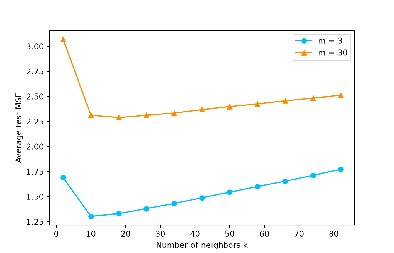
Average test MSE across 50 repetitions for latent dimensions 3 and 30, both observed through 100 covariates.

The m=3m=3 curve has lower average test MSE in this experiment. Averaging a few neighbors reduces noise, while very large neighborhoods blur differences in the regression function. With m=30m=30, even a small neighborhood is less local in the latent variables. The two curves need not have their minima at the same kk. These are simulation averages over independent experiments, not validation scores used to choose a model for a final test set.

c. When m=3m=3, most of the structured variation in 100 covariates is driven by three latent variables. With m=30m=30, distance also responds to many latent directions that do not enter the response. Two observations close in the two relevant latent coordinates may be far apart in those other directions, making Euclidean neighborhoods less useful for predicting YY.

The measurement noise 𝜼i\boldsymbol\eta_i perturbs every observed coordinate and can change which observations are nearest. Without it, 𝑨𝒁i\mathbf A\mathbf Z_i lies in the column space of 𝑨\mathbf A, of dimension at most mm. With independent noise in all 100 coordinates, 𝑿i\mathbf X_i is not confined to that space. Thus the simulation concerns a lower-dimensional signal with noise, not data lying exactly in an mm-dimensional subspace. Keeping the response dependent on two latent variables does not make distances in all observed coordinates equally informative in the two settings.

Question 4: Classify handwritten digits

Original question

Use zip.train and zip.test from the R package ElemStatLearn, as in the lecture. The package has been retired from the active CRAN repository. If needed, install the archived package into your usual R library, then load the two datasets. Python users can use the course copies of the same training data and test data. These compressed CSV files have no headers and are included in the homework ZIP under data/knn. Run the Python code from the folder containing data.

Each image has 16Γ—16=25616\times16=256 pixel values. The first column is the digit label and the remaining columns are the pixel values. Use the first 1,000 rows of zip.train and the first 500 rows of zip.test. Use the original pixel values without standardization, and do not include the digit label in a distance calculation.

For a test image 𝒙0\mathbf x_0 and a training image 𝒙i\mathbf x_i, the two distances are

dE(𝒙0,𝒙i)=βˆ‘j=1256(x0jβˆ’xij)2,dM(𝒙0,𝒙i)=βˆ‘j=1256|x0jβˆ’xij|. d_E(\mathbf x_0,\mathbf x_i) =\sqrt{\sum_{j=1}^{256}(x_{0j}-x_{ij})^2}, \qquad d_M(\mathbf x_0,\mathbf x_i) =\sum_{j=1}^{256}|x_{0j}-x_{ij}|.

  1. Write a 5NN classification function that allows either Euclidean or Manhattan distance. For each test image, calculate its distances to the training images directly, find the five nearest, and return the most frequent digit label. Break distance ties by the smaller training row number and voting ties by the smallest digit. Do not use a built-in distance or KNN function for this part.

  2. Apply the classifier to all 500 test images using each distance. For each fit, report the test classification error and a 10Γ—1010\times10 confusion matrix, with rows representing predicted digits and columns representing true digits. Keep all digit labels from 0 through 9 in the matrix, including any with a zero count. Which digits are most often confused with one another?

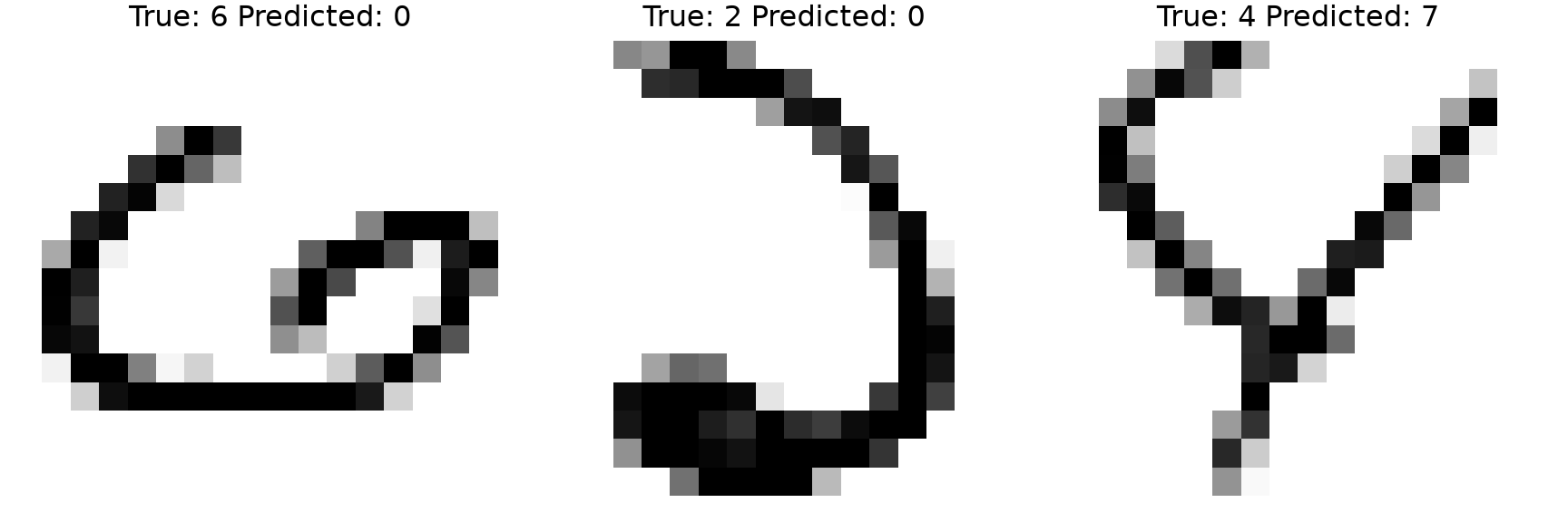
  3. For Euclidean distance, display three incorrectly classified test images, together with their true and predicted labels. Comment on whether the mistakes are visually understandable. Compare the overall results of the two distance measures. Can they have similar total error while making mistakes on different images? Use your predictions to support your answer.

Solution

With the specified training and test rows, Euclidean 5NN makes 61 errors out of 500, and Manhattan 5NN makes 69. Both recognize most digits, but some of their errors occur on different images.

a. Write the classifier. For each test image, calculate the distances, sort the training rows, and count the labels of the five closest images. Passing either of the distance functions below changes the distance without changing the remaining classification rule.

  • R
  • Python
Show the solution code
library(ElemStatLearn)

euclidean_distance <- function(x0, X) {
  sqrt(rowSums(sweep(X, 2, x0, "-")^2))
}

manhattan_distance <- function(x0, X) {
  rowSums(abs(sweep(X, 2, x0, "-")))
}

X <- zip.train[1:1000, -1]
y <- zip.train[1:1000, 1]
X_test <- zip.test[1:500, -1]
y_test <- zip.test[1:500, 1]

knn_classify <- function(X, y, X_test, distance) {
  y_hat <- integer(nrow(X_test))
  for (i in seq_len(nrow(X_test))) {
    d <- distance(X_test[i, ], X)
    neighbors <- order(d, seq_len(nrow(X)))[1:5]
    y_hat[i] <- which.max(tabulate(y[neighbors] + 1, nbins = 10)) - 1
  }
  y_hat
}

y_hat <- cbind(Euclidean = knn_classify(X, y, X_test, euclidean_distance),
               Manhattan = knn_classify(X, y, X_test, manhattan_distance))
Show the solution code
import numpy as np
import pandas as pd
import matplotlib.pyplot as plt

zip_train = np.loadtxt("data/knn/zip-train.csv.gz", delimiter=",")
zip_test = np.loadtxt("data/knn/zip-test.csv.gz", delimiter=",")

def euclidean_distance(x0, X):
    return np.sqrt(np.sum((X - x0)**2, axis=1))

def manhattan_distance(x0, X):
    return np.sum(np.abs(X - x0), axis=1)

X = zip_train[:1000, 1:]
y = zip_train[:1000, 0].astype(int)
X_test = zip_test[:500, 1:]
y_test = zip_test[:500, 0].astype(int)

def knn_classify(X, y, X_test, distance):
    y_hat = np.zeros(X_test.shape[0], dtype=int)
    for i in range(X_test.shape[0]):
        d = distance(X_test[i], X)
        neighbors = np.argsort(d, kind="stable")[:5]
        y_hat[i] = np.argmax(np.bincount(y[neighbors], minlength=10))
    return y_hat

y_hat = np.column_stack((knn_classify(X, y, X_test, euclidean_distance),
                          knn_classify(X, y, X_test, manhattan_distance)))

b. Evaluate classification. Each column of y_hat contains 500 predictions. The confusion matrices below have predicted digits in rows and true digits in columns.

  • R
  • Python
Show the solution code
for (l in 1:2) {
  cat(colnames(y_hat)[l], "test error:", mean(y_hat[, l] != y_test), "\n")
  print(table(Predicted = factor(y_hat[, l], levels = 0:9),
              True = factor(y_test, levels = 0:9)))
}
Euclidean test error: 0.122 
         True
Predicted   0   1   2   3   4   5   6   7   8   9
        0 118   0   7   1   0   4   2   0   2   0
        1   0  66   0   0   2   0   0   0   0   1
        2   0   0  39   1   0   0   2   0   0   1
        3   0   0   0  23   0   4   0   0   2   0
        4   0   0   1   0  27   1   1   1   0   1
        5   0   0   0   1   0  13   0   0   0   0
        6   0   2   0   0   0   1  41   0   2   0
        7   0   0   0   0   1   1   0  34   0   4
        8   0   0   3   2   0   2   0   0  37   0
        9   1   0   0   1   4   0   0   1   1  41
Manhattan test error: 0.138 
         True
Predicted   0   1   2   3   4   5   6   7   8   9
        0 118   0   6   1   0   5   3   0   4   0
        1   0  67   2   0   2   0   1   0   0   1
        2   0   0  35   0   0   0   2   0   0   0
        3   0   0   1  24   0   4   0   0   2   0
        4   0   0   1   1  27   1   0   1   0   1
        5   0   0   0   1   0  11   0   0   0   0
        6   0   1   0   0   0   2  40   0   2   0
        7   0   0   2   1   1   0   0  34   0   5
        8   0   0   2   0   0   3   0   0  34   0
        9   1   0   1   1   4   0   0   1   2  41
Show the solution code
for l in range(2):
    print(["Euclidean", "Manhattan"][l],
          "test error:", np.mean(y_hat[:, l] != y_test))
    print(pd.crosstab(pd.Series(y_hat[:, l], name="Predicted"),
                      pd.Series(y_test, name="True"))
          .reindex(index=range(10), columns=range(10), fill_value=0))
Euclidean test error: 0.122
True         0   1   2   3   4   5   6   7   8   9
Predicted                                         
0          118   0   7   1   0   4   2   0   2   0
1            0  66   0   0   2   0   0   0   0   1
2            0   0  39   1   0   0   2   0   0   1
3            0   0   0  23   0   4   0   0   2   0
4            0   0   1   0  27   1   1   1   0   1
5            0   0   0   1   0  13   0   0   0   0
6            0   2   0   0   0   1  41   0   2   0
7            0   0   0   0   1   1   0  34   0   4
8            0   0   3   2   0   2   0   0  37   0
9            1   0   0   1   4   0   0   1   1  41
Manhattan test error: 0.138
True         0   1   2   3   4   5   6   7   8   9
Predicted                                         
0          118   0   6   1   0   5   3   0   4   0
1            0  67   2   0   2   0   1   0   0   1
2            0   0  35   0   0   0   2   0   0   0
3            0   0   1  24   0   4   0   0   2   0
4            0   0   1   1  27   1   0   1   0   1
5            0   0   0   1   0  11   0   0   0   0
6            0   1   0   0   0   2  40   0   2   0
7            0   0   2   1   1   0   0  34   0   5
8            0   0   2   0   0   3   0   0  34   0
9            1   0   1   1   4   0   0   1   2  41

The test error is 0.122 for Euclidean distance and 0.138 for Manhattan distance. The most frequent individual confusion is a true 2 predicted as 0: seven images under Euclidean distance and six under Manhattan distance. Other frequent errors include 5 predicted as 0 or 3, 9 predicted as 7, and 4 predicted as 9. These are counts for this test set, whose digit classes have different sample sizes.

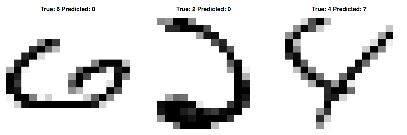
c. Inspect mistakes and compare predictions. We display the first three Euclidean errors, keeping the lecture’s image orientation.

  • R
  • Python
Show the solution code
incorrect <- which(y_hat[, 1] != y_test)[1:3]
old_par <- par(mfrow = c(1, 3), mar = c(1, 1, 3, 1))
for (i in incorrect) {
  image(zip2image(zip.test, i), col = gray(256:0/256), zlim = c(0, 1),
        xlab = "", ylab = "", axes = FALSE,
        main = paste("True:", y_test[i], "Predicted:", y_hat[i, 1]))
}
[1] "digit  6  taken"
[1] "digit  2  taken"
[1] "digit  4  taken"

Show the solution code
par(old_par)

cat("Different predictions:", sum(y_hat[, 1] != y_hat[, 2]), "\n")
Different predictions: 22 
Show the solution code
table(Euclidean_correct = y_hat[, 1] == y_test,
      Manhattan_correct = y_hat[, 2] == y_test)
                 Manhattan_correct
Euclidean_correct FALSE TRUE
            FALSE    58    3
            TRUE     11  428
Show the solution code
incorrect = np.flatnonzero(y_hat[:, 0] != y_test)[:3]
plt.figure(figsize=(9, 3))
for l in range(3):
    i = incorrect[l]
    plt.subplot(1, 3, l + 1)
    plt.imshow(zip_test[i, 1:].reshape(16, 16), cmap="gray_r",
               vmin=0, vmax=1, interpolation="nearest")
    plt.title(f"True: {y_test[i]} Predicted: {y_hat[i, 0]}")
    plt.axis("off")
plt.tight_layout()
plt.show()

Show the solution code
print("Different predictions:", np.sum(y_hat[:, 0] != y_hat[:, 1]))
Different predictions: 22
Show the solution code
print(pd.crosstab(pd.Series(y_hat[:, 0] == y_test, name="Euclidean correct"),
                  pd.Series(y_hat[:, 1] == y_test, name="Manhattan correct")))
Manhattan correct  False  True 
Euclidean correct              
False                 58      3
True                  11    428

These images are test rows 4, 13, and 14, with true labels 6, 2, and 4, but predicted labels 0, 0, and 7. The 6 has a rounded lower loop, the 2 has an unusually curved outline, and the 4 lacks a typical horizontal crossbar. These shapes make pixel-distance mistakes plausible, even when a person can recognize the digit. Visual recognition also uses information about handwriting that this distance rule does not explicitly represent.

The methods disagree on 22 predicted labels. Euclidean distance is correct and Manhattan distance is wrong on 11 images; the reverse happens on three. On eight additional images, both are wrong but predict different digits. Thus, similar total errors can hide different mistakes. Euclidean distance has the smaller error on this split, but this comparison does not establish that it will always be better.

Question 5: Create a plot-formatting skill

Original question

Create a short SKILL.md file for improving the formatting of STAT 432 homework plots. You may use AI to help write it.

  1. Include a title, a description, and a few formatting rules. The description should limit the skill to STAT 432 homework plot improvements and require an explicit request to use it. Your rules should address margins, titles, axes, labels, colors, and sizes for plots produced in R or Python. Keep them portable: do not refer to specific homework questions.

  2. Ask your agent to install the skill. Explicitly call it to improve the plot from Question 1, then compare the original and revised versions. Do you like the changes? You may revise the skill and test it a couple more times, or uninstall it if it remains unhelpful.

  3. Append your final SKILL.md content to your submission and briefly explain your choices and experience.

Solution

There is no single correct visual style. The following is one possible SKILL.md:

---
name: format-homework-plots
description: Use only when the user explicitly calls this skill to improve the formatting of a STAT 432 homework plot.
---

# STAT 432 Plot Formatting

- Preserve the plotted data, calculations, and statistical meaning.
- Leave enough margin for titles, axis labels, tick labels, and legends without clipping.
- Use a short, informative title.
- Label axes clearly, include units when relevant, and use readable tick spacing and labels.
- Use a colorblind-friendly palette and distinguish curves with line styles when helpful.
- Start with a 6.5 by 4.5 inch figure, 12-point labels, and a 14-point title; adjust for multiple panels.
- Apply these rules to the existing R or Python plotting code.

The title identifies the skill, and the description limits both its scope and when it should be used. The rules express reusable formatting preferences without referring to an individual homework question. Figure and font sizes provide a starting point that can be revised after viewing the result.

Save the file as format-homework-plots/SKILL.md and ask your agent to install it. An explicit test request is: β€œUse format-homework-plots to improve the formatting of my Question 1 plot.”

Compare the original and revised plots in your report. Describe the actual changes, whether they make the plot easier to read, and which preferences you revised or kept. Keeping, revising, or uninstalling the skill can all be reasonable outcomes; the explanation should reflect your own test.

STAT 432 | Basics of Statistical Learning

 
  • Instructor