Homework 04 Solutions

Before you begin

Each solution repeats the complete question before presenting the reasoning. All four questions include both R and Python code, but students need to use only one language. Questions 1 through 3 use the same models and objectives but generate different random observations, so their exact numerical results need not agree. Question 2 uses the same seed as Question 1, so within each language the 200 datasets are the same in both questions; only the fitting method changes. Question 4 uses the same observations, split, and folds in both languages, but package-specific penalty grids and fitting conventions can give different tuning results.

Download the materials

The ZIP file contains the two editable QMD files. The solution code generates all simulation results and figures.

Question 1: Signal strength and correlated substitutes

Original question

Consider a regression problem with $n=120$ observations and $p=10$ covariates. Create one simulated dataset as follows. Generate the first covariate $X_1$ as $n$ independent standard normal draws. Then form the second covariate as

$X_2 = 0.999X_1 + \sqrt{1-0.999^2}\,Z,$

where $Z$ is another vector of $n$ independent standard normal draws, so that $X_1$ and $X_2$ have population correlation $0.999$ . Generate the remaining covariates $X_3,\ldots,X_{10}$ as independent standard normal vectors of length $n$ .

Thus $X_1$ and $X_2$ are extremely highly correlated, while $X_3$ and $X_4$ are independent of one another and of the remaining covariates. Finally, generate the response as

$Y = 0.15X_1 +0.15X_2 +0.30X_3 +0.15X_4 +\epsilon,$

where $\epsilon$ is a vector of $n$ independent standard normal errors, independent of the covariates. Both members of the correlated pair appear in the generating equation with the same coefficient, even though each one carries almost the same observed information as the other. The two independent signals $X_3$ and $X_4$ have coefficients that differ by a factor of two, and $X_5,\ldots,X_{10}$ have zero coefficients.

Use seed 43246 and independently repeat the complete data generation and fitting procedure 200 times. Within each repetition, center and standardize the covariates using divisor $n$ and center the response. Fit the lasso model with the glmnet package in R or sklearn.linear_model.Lasso in Python, without scaling the variables inside the fitting function, at

$\lambda\in\{0.08,0.12,0.18,0.24\}.$

Make sure you understand which argument specifies the scaling option in a lasso fit and how to give a specific penalty value; the default settings of the fitting function do not produce the fits required here.

Fit all four penalties to the same generated dataset before beginning the next repetition. Leave the intercept unpenalized and convert the fitted slopes back to the original covariate scale. Store the slopes in one array whose dimensions correspond to the 200 repetitions, 10 covariates, and four penalties. Treat a slope as nonzero when its absolute value exceeds $10^{-8}$ . Use a tight convergence tolerance as well as a sufficiently large iteration limit, because the nearly identical covariates make coefficient allocation sensitive to numerical accuracy. In R, use control = list(thresh = 1e-18, maxit = 1000000); in Python, use tol=1e-10, max_iter=100000. Verify that all 800 fits converge. R and Python use different random-number generators, so their exact numerical results need not agree.

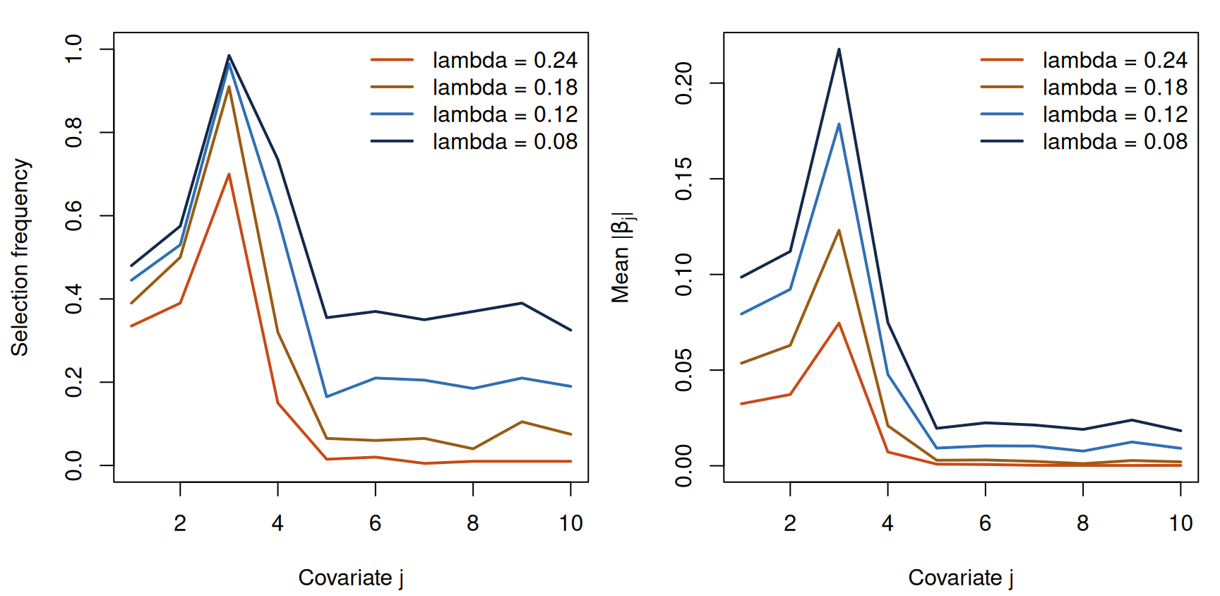
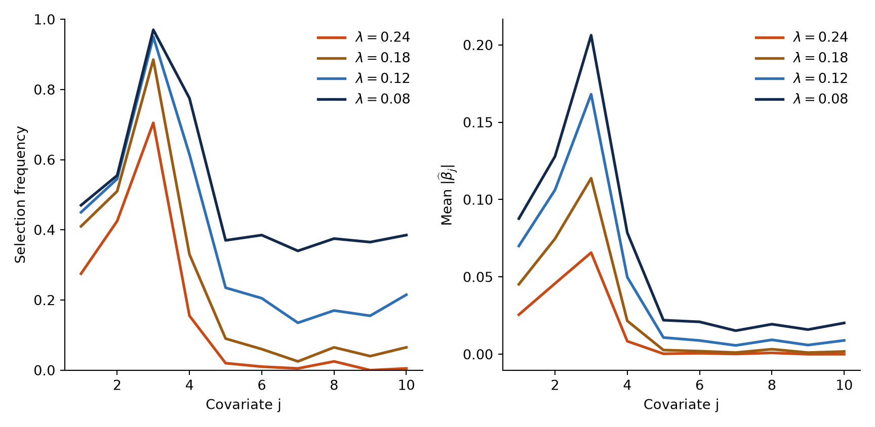
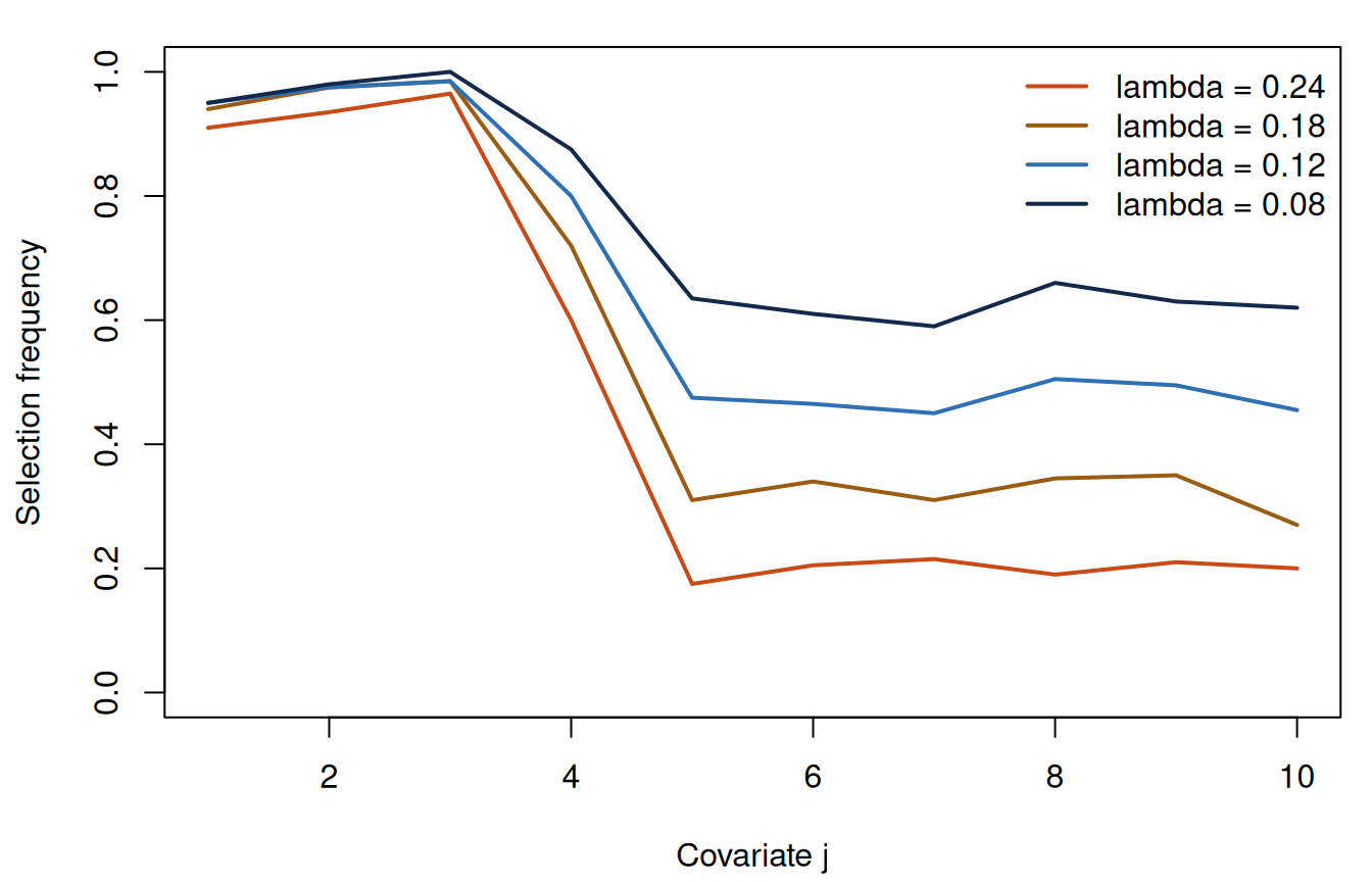
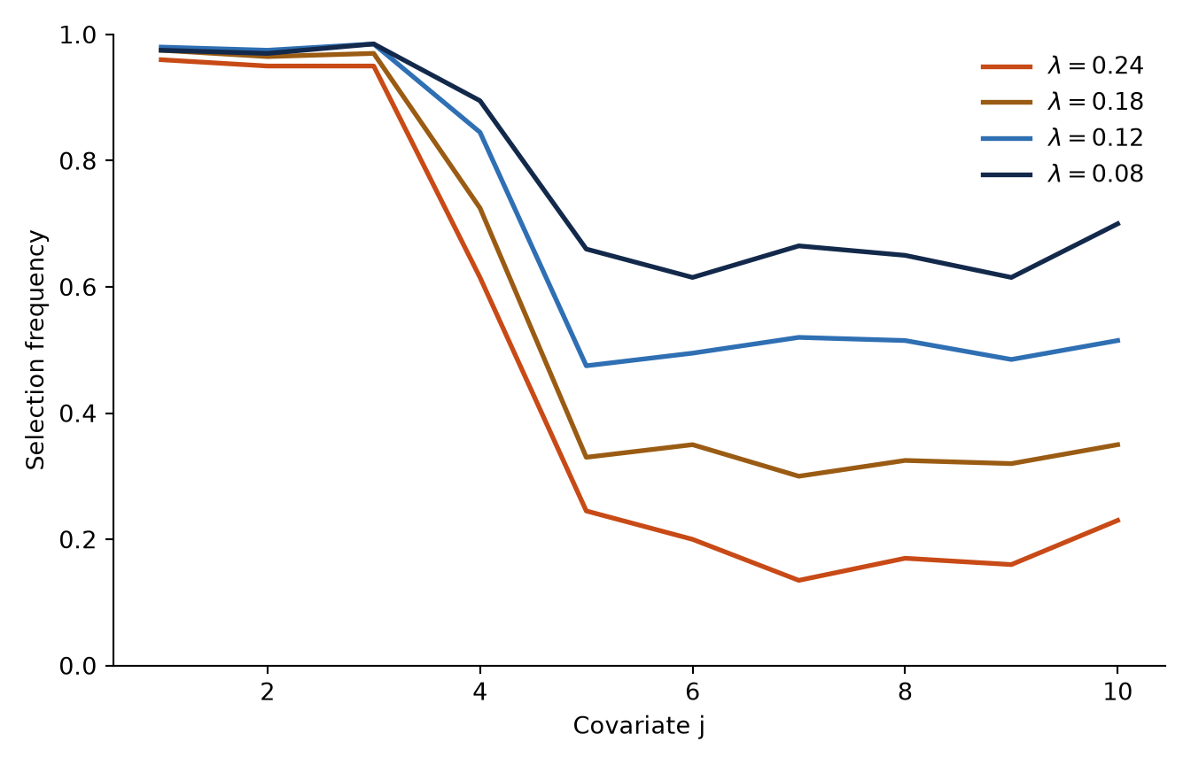
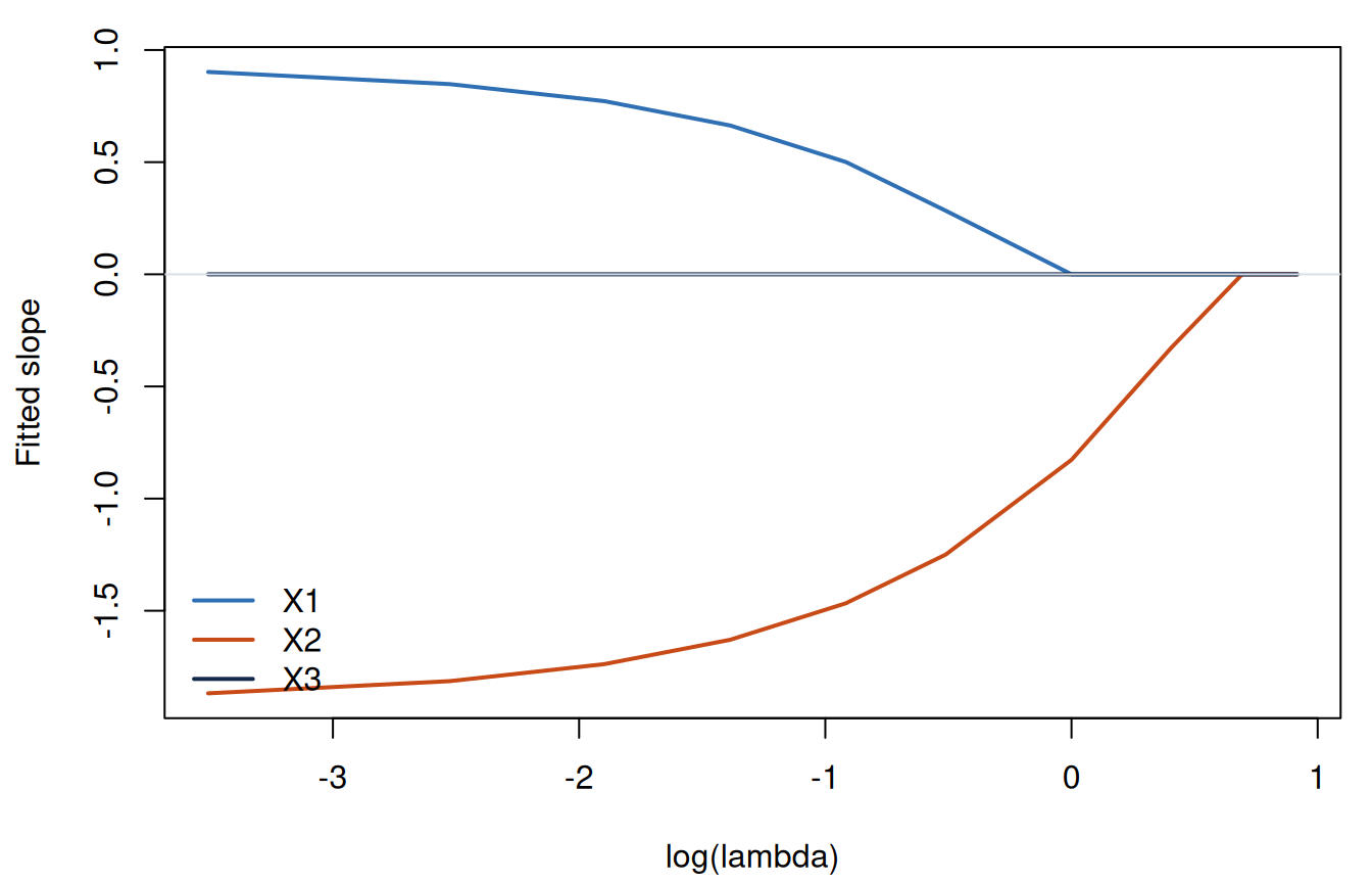
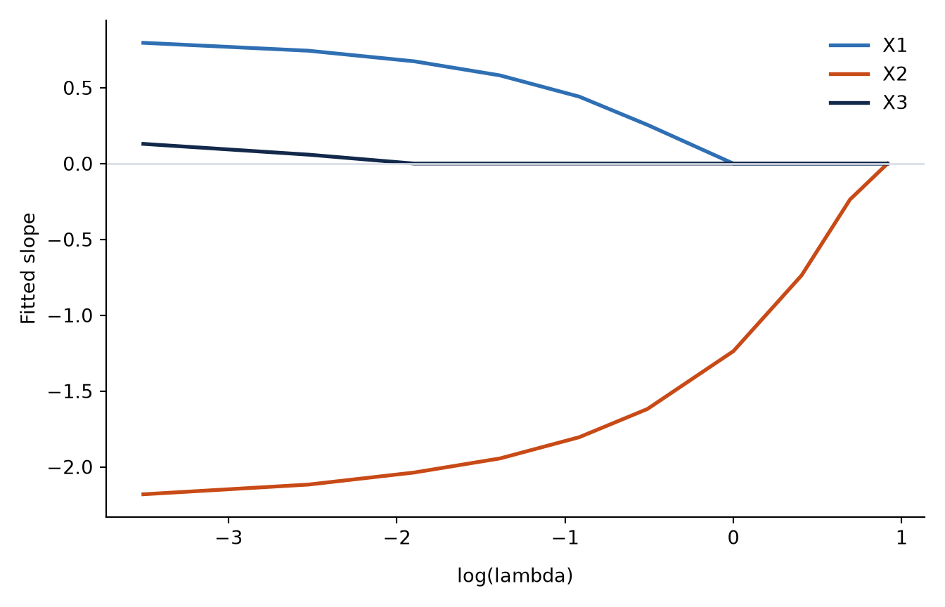
For every covariate and penalty, report the selection frequency and the mean absolute fitted slope, where the mean includes fitted zeros. Draw one figure for each summary. Explain how increasing the penalty changes the fitted magnitudes and selection frequencies.
For the pair $(X_1,X_2)$ , report the frequency of four mutually exclusive outcomes at each penalty: only the first covariate is selected, only the second is selected, both are selected, and neither is selected. Compare the two marginal selection frequencies and explain why they are similar. Describe how the four outcomes shift as the penalty increases, and explain why lasso can produce a sparse fitted rule that omits one member of the pair even though both members appear in the generating equation.
Compare the selection frequencies of $X_3$ and $X_4$ with the average selection frequency among $X_5,\ldots,X_{10}$ . Explain how signal magnitude and the penalty account for the pattern. Use the correlated pair to explain why a fitted zero does not establish that the corresponding population coefficient is zero, and why a nonzero fitted coefficient does not establish that the variable is uniquely important.

Solution

Read the design before coding. The correlated pair contributes approximately $(0.15+0.15\times0.999)\,X_1\approx0.30X_1$ to the mean, so its combined signal is comparable to the independent signal $X_3$ with coefficient $0.30$ , while $X_4$ at $0.15$ is weaker. Every covariate is generated with population variance one, so the learned scales are close to one in every repetition; the code still learns the centers and scales from the current repetition and converts the fitted slopes back, as the question requires.

The package calls must match the stated preprocessing. In glmnet, the scaling option is standardize, and the fits below use standardize = FALSE because the columns are already standardized with divisor $n$ ; intercept = FALSE because the response is already centered; and the penalty grid is supplied through lambda. In scikit-learn, Lasso never standardizes its input, fit_intercept = FALSE plays the same role, and the penalty is supplied through alpha. With these choices, both packages minimize $\lVert\widetilde{\mathbf y}-\mathbf X\boldsymbol\beta\rVert_2^2/(2n)+\lambda\lVert\boldsymbol\beta\rVert_1$ on the manually prepared data.

Show the solution code

library(glmnet)

set.seed(43246)
n <- 120
p <- 10
n_simulations <- 200
beta <- c(0.15, 0.15, 0.30, 0.15, rep(0, 6))

# Fit the penalties in decreasing order with warm starts.
lambda_values <- c(0.24, 0.18, 0.12, 0.08)
beta_hat <- array(0, dim = c(n_simulations, p, length(lambda_values)))
sample_correlation <- numeric(n_simulations)

for (k in seq_len(n_simulations)) {
  U <- matrix(rnorm(n * p), nrow = n, ncol = p)
  X <- U
  X[, 2] <- 0.999 * U[, 1] + sqrt(1 - 0.999^2) * U[, 2]
  y <- drop(X %*% beta) + rnorm(n)

  sample_correlation[k] <- cor(X[, 1], X[, 2])

  # Center and standardize with divisor n; the package must not rescale.
  x_bar <- colMeans(X)
  X_centered <- sweep(X, 2, x_bar, "-")
  s <- sqrt(colMeans(X_centered^2))
  X_std <- sweep(X_centered, 2, s, "/")
  y_centered <- y - mean(y)

  fit <- glmnet(
    X_std, y_centered,
    alpha = 1, lambda = lambda_values,
    standardize = FALSE, intercept = FALSE,
    # Tight tolerance matters for coefficient allocation at correlation 0.999.
    control = list(thresh = 1e-18, maxit = 1000000)
  )
  stopifnot(
    fit$jerr == 0,
    isTRUE(all.equal(fit$lambda, lambda_values)),
    all(is.finite(fit$beta))
  )

  # Convert the fitted slopes back to the original covariate scale.
  beta_hat[k, , ] <- sweep(as.matrix(fit$beta), 1, s, "/")
}

selected <- abs(beta_hat) > 1e-8
selection_frequency <- apply(selected, c(2, 3), mean)
mean_magnitude <- apply(abs(beta_hat), c(2, 3), mean)

Show the solution code

# Tabulate selection frequencies and mean magnitudes per covariate and penalty.
selection_table <- data.frame(
  covariate = paste0("X", seq_len(p)),
  selection_frequency,
  check.names = FALSE
)
names(selection_table)[-1] <- paste0("lambda_", lambda_values)
magnitude_table <- data.frame(
  covariate = paste0("X", seq_len(p)),
  mean_magnitude,
  check.names = FALSE
)
names(magnitude_table)[-1] <- paste0("lambda_", lambda_values)

knitr::kable(selection_table, digits = 3)

covariate	lambda_0.24	lambda_0.18	lambda_0.12	lambda_0.08
X1	0.335	0.390	0.445	0.480
X2	0.390	0.500	0.530	0.575
X3	0.700	0.910	0.965	0.985
X4	0.150	0.320	0.595	0.735
X5	0.015	0.065	0.165	0.355
X6	0.020	0.060	0.210	0.370
X7	0.005	0.065	0.205	0.350
X8	0.010	0.040	0.185	0.370
X9	0.010	0.105	0.210	0.390
X10	0.010	0.075	0.190	0.325

Selection frequencies and mean absolute fitted slopes across 200 lasso simulations.

Show the solution code

knitr::kable(magnitude_table, digits = 3)

covariate	lambda_0.24	lambda_0.18	lambda_0.12	lambda_0.08
X1	0.032	0.054	0.079	0.099
X2	0.037	0.063	0.092	0.112
X3	0.075	0.123	0.179	0.218
X4	0.007	0.021	0.048	0.075
X5	0.001	0.003	0.009	0.020
X6	0.001	0.003	0.010	0.022
X7	0.000	0.002	0.010	0.021
X8	0.000	0.001	0.008	0.019
X9	0.000	0.003	0.012	0.024
X10	0.000	0.002	0.009	0.018

Selection frequencies and mean absolute fitted slopes across 200 lasso simulations.

Show the solution code

# Draw the two summaries side by side for the four penalties.
curve_colors <- c("#C84A16", "#9A5B13", "#2F6FB3", "#13294B")
old_par <- par(no.readonly = TRUE)
par(mfrow = c(1, 2), mar = c(4.2, 4.2, 1.2, 0.8))
matplot(
  seq_len(p), selection_frequency,
  type = "l", lty = 1, lwd = 2, col = curve_colors,
  ylim = c(0, 1), xlab = "Covariate j", ylab = "Selection frequency"
)
legend(
  "topright", legend = paste("lambda =", lambda_values),
  col = curve_colors, lty = 1, lwd = 2, bty = "n"
)
matplot(
  seq_len(p), mean_magnitude,
  type = "l", lty = 1, lwd = 2, col = curve_colors,
  xlab = "Covariate j",
  ylab = expression("Mean " * "|" * hat(beta)[j] * "|")
)
legend(
  "topright", legend = paste("lambda =", lambda_values),
  col = curve_colors, lty = 1, lwd = 2, bty = "n"
)

Two panels compare ten covariates at four penalty values. The highly correlated first pair has similar selection frequencies, the third and fourth covariates stand above the noise covariates, and all magnitudes decrease under stronger penalties. — Selection frequencies and mean absolute fitted slopes across 200 lasso simulations.

Show the solution code

par(old_par)

Show the solution code

# Tally the four mutually exclusive selection outcomes for the pair.
pair_outcomes <- matrix(
  NA_real_,
  nrow = length(lambda_values),
  ncol = 4
)
for (l in seq_along(lambda_values)) {
  selected_l <- selected[, , l]
  pair_outcomes[l, ] <- c(
    mean(selected_l[, 1] & !selected_l[, 2]),
    mean(!selected_l[, 1] & selected_l[, 2]),
    mean(selected_l[, 1] & selected_l[, 2]),
    mean(!selected_l[, 1] & !selected_l[, 2])
  )
}
pair_outcomes <- data.frame(
  lambda = lambda_values,
  pair_outcomes,
  check.names = FALSE
)
names(pair_outcomes)[-1] <- c("X1 only", "X2 only", "both", "neither")

# Compare the two independent signals with the noise average.
signal_comparison <- data.frame(
  lambda = lambda_values,
  X3 = selection_frequency[3, ],
  X4 = selection_frequency[4, ],
  mean_X5_to_X10 = colMeans(selection_frequency[5:10, , drop = FALSE])
)

knitr::kable(pair_outcomes, digits = 3)

lambda	X1 only	X2 only	both	neither
0.24	0.315	0.370	0.02	0.295
0.18	0.370	0.480	0.02	0.130
0.12	0.415	0.500	0.03	0.055
0.08	0.410	0.505	0.07	0.015

Show the solution code

knitr::kable(signal_comparison, digits = 3)

lambda	X3	X4	mean_X5_to_X10
0.24	0.700	0.150	0.012
0.18	0.910	0.320	0.068
0.12	0.965	0.595	0.194
0.08	0.985	0.735	0.360

Show the solution code

round(c(
  mean_correlation = mean(sample_correlation),
  minimum_correlation = min(sample_correlation),
  maximum_correlation = max(sample_correlation)
), 5)

   mean_correlation minimum_correlation maximum_correlation 
            0.99899             0.99833             0.99943

Show the solution code

import numpy as np
import pandas as pd
from sklearn.linear_model import Lasso

rng = np.random.default_rng(43246)
n = 120
p = 10
n_simulations = 200
beta = np.array([0.15, 0.15, 0.30, 0.15, 0, 0, 0, 0, 0, 0.0])

# Fit the penalties in decreasing order with warm starts.
lambda_values = np.array([0.24, 0.18, 0.12, 0.08])

beta_hat = np.zeros((n_simulations, p, len(lambda_values)))
sample_correlation = np.empty(n_simulations)
iterations = np.empty((n_simulations, len(lambda_values)), dtype=int)
max_iterations = 100000

for k in range(n_simulations):
    U = rng.normal(size=(n, p))
    X = U.copy()
    X[:, 1] = 0.999 * U[:, 0] + np.sqrt(1 - 0.999**2) * U[:, 1]
    y = X @ beta + rng.normal(size=n)

    sample_correlation[k] = np.corrcoef(X[:, 0], X[:, 1])[0, 1]

    # Center and standardize with divisor n; the package must not rescale.
    x_bar = X.mean(axis=0)
    X_centered = X - x_bar
    s = np.sqrt(np.mean(X_centered**2, axis=0))
    X_std = X_centered / s
    y_centered = y - y.mean()

    fit = Lasso(
        fit_intercept=False,
        warm_start=True,
        max_iter=max_iterations,
        tol=1e-10,
        selection="cyclic",
    )
    for l, lam in enumerate(lambda_values):
        fit.set_params(alpha=lam)
        fit.fit(X_std, y_centered)
        # Convert the fitted slopes back to the original covariate scale.
        beta_hat[k, :, l] = fit.coef_ / s
        iterations[k, l] = fit.n_iter_

assert np.all(iterations < max_iterations)
selected = np.abs(beta_hat) > 1e-8
selection_frequency = selected.mean(axis=0)
mean_magnitude = np.abs(beta_hat).mean(axis=0)

Show the solution code

import matplotlib.pyplot as plt

# Tabulate selection frequencies and mean magnitudes per covariate and penalty.
selection_table = pd.DataFrame(
    selection_frequency,
    index=[f"X{j}" for j in range(1, p + 1)],
    columns=[f"lambda_{lam}" for lam in lambda_values],
)
magnitude_table = pd.DataFrame(
    mean_magnitude,
    index=[f"X{j}" for j in range(1, p + 1)],
    columns=[f"lambda_{lam}" for lam in lambda_values],
)
print(selection_table.round(3).to_string())

     lambda_0.24  lambda_0.18  lambda_0.12  lambda_0.08
X1         0.275        0.410        0.450        0.470
X2         0.425        0.510        0.545        0.555
X3         0.705        0.885        0.950        0.970
X4         0.155        0.330        0.615        0.775
X5         0.020        0.090        0.235        0.370
X6         0.010        0.060        0.205        0.385
X7         0.005        0.025        0.135        0.340
X8         0.025        0.065        0.170        0.375
X9         0.000        0.040        0.155        0.365
X10        0.005        0.065        0.215        0.385

Show the solution code

print(magnitude_table.round(3).to_string())

     lambda_0.24  lambda_0.18  lambda_0.12  lambda_0.08
X1         0.026        0.045        0.070        0.088
X2         0.046        0.075        0.106        0.128
X3         0.066        0.114        0.168        0.206
X4         0.008        0.022        0.050        0.079
X5         0.000        0.003        0.011        0.022
X6         0.001        0.002        0.009        0.021
X7         0.000        0.001        0.006        0.015
X8         0.001        0.003        0.009        0.019
X9         0.000        0.001        0.006        0.016
X10        0.000        0.002        0.009        0.020

Show the solution code

# Draw the two summaries side by side for the four penalties.
curve_colors = ["#C84A16", "#9A5B13", "#2F6FB3", "#13294B"]
fig, axes = plt.subplots(1, 2, figsize=(9, 4.4))
for l, (lam, color) in enumerate(zip(lambda_values, curve_colors)):
    axes[0].plot(
        np.arange(1, p + 1), selection_frequency[:, l],
        color=color, linewidth=2, label=rf"$\lambda={lam}$",
    )
    axes[1].plot(
        np.arange(1, p + 1), mean_magnitude[:, l],
        color=color, linewidth=2, label=rf"$\lambda={lam}$",
    )
axes[0].set(
    xlabel="Covariate j", ylabel="Selection frequency", ylim=(0, 1)
)
axes[1].set(xlabel="Covariate j", ylabel=r"Mean $|\widehat\beta_j|$")
for ax in axes:
    ax.legend(frameon=False)
    ax.spines[["top", "right"]].set_visible(False)
fig.tight_layout()
plt.show()

Show the solution code

# Tally the four mutually exclusive selection outcomes for the pair.
pair_outcomes = []
for l, lam in enumerate(lambda_values):
    selected_l = selected[:, :, l]
    pair_outcomes.append({
        "lambda": lam,
        "X1 only": np.mean(selected_l[:, 0] & ~selected_l[:, 1]),
        "X2 only": np.mean(~selected_l[:, 0] & selected_l[:, 1]),
        "both": np.mean(selected_l[:, 0] & selected_l[:, 1]),
        "neither": np.mean(~selected_l[:, 0] & ~selected_l[:, 1]),
    })
pair_outcomes = pd.DataFrame(pair_outcomes)

# Compare the two independent signals with the noise average.
signal_comparison = pd.DataFrame({
    "lambda": lambda_values,
    "X3": selection_frequency[2],
    "X4": selection_frequency[3],
    "mean_X5_to_X10": selection_frequency[4:10].mean(axis=0),
})
print(pair_outcomes.round(3).to_string(index=False))

 lambda  X1 only  X2 only  both  neither
   0.24     0.27    0.420 0.005    0.305
   0.18     0.40    0.500 0.010    0.090
   0.12     0.43    0.525 0.020    0.025
   0.08     0.44    0.525 0.030    0.005

Show the solution code

print(signal_comparison.round(3).to_string(index=False))

 lambda    X3    X4  mean_X5_to_X10
   0.24 0.705 0.155           0.011
   0.18 0.885 0.330           0.057
   0.12 0.950 0.615           0.186
   0.08 0.970 0.775           0.370

Show the solution code

print(pd.Series({
    "mean_correlation": sample_correlation.mean(),
    "minimum_correlation": sample_correlation.min(),
    "maximum_correlation": sample_correlation.max(),
}).round(5).to_string())

mean_correlation       0.99899
minimum_correlation    0.99845
maximum_correlation    0.99939

As a check of the data generation, the sample correlation between $X_1$ and $X_2$ stays between $0.998$ and $0.9995$ in every repetition of both language runs. All 800 fits converge in each language: R verifies jerr == 0 and the requested penalty grid, while Python asserts that every fit stops below the iteration limit.

a. Increasing the penalty lowers every selection frequency and every mean absolute fitted slope. At $\lambda=0.12$ , for example, the R run selects $X_3$ in $96.5\%$ of the repetitions, $X_4$ in $59.5\%$ , each member of the correlated pair in about half, and the noise covariates in $19\%$ on average; the Python run gives $95\%$ , $61.5\%$ , about half, and $18.6\%$ . At the strongest penalty $\lambda=0.24$ , the noise average falls to about $1\%$ in both runs, while $X_3$ is still selected about $70\%$ of the time. The mean absolute slopes show the same attenuation: soft thresholding subtracts $\lambda$ from each surviving coordinate score, so fitted magnitudes shrink toward zero as the penalty grows. Individual coefficient paths need not decrease monotonically under correlation, but the across-repetition summaries do.

b. The pair outcomes at $\lambda=0.12$ in the R run are: only $X_1$ in $41.5\%$ , only $X_2$ in $50.0\%$ , both in $3.0\%$ , and neither in $5.5\%$ of the repetitions. Python gives $43.0\%$ , $52.5\%$ , $2.0\%$ , and $2.5\%$ . The two marginal selection frequencies are similar because the construction treats the two covariates symmetrically: they have the same population coefficient, the same marginal distribution, and an exchangeable joint distribution, so neither is systematically preferred. The remaining gap is consistent with Monte Carlo variation: the difference of two disjoint outcome proportions over 200 repetitions carries a standard error of roughly $\sqrt{(0.415+0.500)/200}\approx0.07$ .

The four outcomes shift with the penalty in a consistent direction. As $\lambda$ decreases, “neither” disappears (from about $30\%$ at $\lambda=0.24$ to almost zero at $\lambda=0.08$ ) and single-member fits dominate; “both” remains uncommon at every penalty. Once one member represents the shared direction, the partial residual seen by the other member carries little remaining signal, so the coordinate updates keep one sparse representative rather than splitting the effect. This is why a fitted rule can omit $X_1$ or $X_2$ even though both coefficients are nonzero in the generating equation: the omitted member’s information is carried almost perfectly by its substitute. At least one member is selected about $95\%$ to $98\%$ of the time at $\lambda=0.12$ , close to the selection frequency of $X_3$ , whose coefficient equals the pair’s combined effect.

c. The two independent signals separate cleanly by strength. At $\lambda=0.12$ , $X_3$ (coefficient $0.30$ ) is selected about $95$ – $97\%$ of the time, while $X_4$ (coefficient $0.15$ ) is selected about $60\%$ ; the noise covariates average about $19\%$ and fall to about $1\%$ at $\lambda=0.24$ . For a covariate that is independent of the others, the score is centered near its population coefficient with spread about $1/\sqrt{n}$ , so the weaker coefficient $0.15$ leaves its score inside the threshold interval $[-\lambda,\lambda]$ more often than the stronger coefficient $0.30$ , and a larger penalty widens that interval. The correlated pair behaves differently: each member’s score also reflects the other member’s contribution, so both scores are centered near the combined effect rather than the individual coefficient $0.15$ .

The pair supplies the two interpretation cautions. First, a fitted zero does not establish a zero population coefficient: each member of the pair has a true coefficient of $0.15$ , yet at $\lambda=0.12$ each is omitted in about half of the repetitions. Second, a nonzero fitted coefficient does not establish that the variable is uniquely important: the selected member of the pair is standing in for information shared with a covariate that the same fitted rule may omit. Selection in one sample describes one sparse predictive rule, not the structure of the generating equation.

Question 2: Elastic net with an equal penalty mix

Original question

This question continues the simulation of Question 1. Generate the data exactly as in Question 1, with the same seed 43246, so that the 200 repetitions produce the same datasets and the only change is the fitting method. Now fit the elastic net model with mixing parameter $\alpha=0.5$ , which places equal weight on the $\ell_1$ and squared $\ell_2$ penalties. Use the glmnet package in R or sklearn.linear_model.ElasticNet in Python, with the same four penalties $\lambda\in\{0.08,0.12,0.18,0.24\}$ and the same fitting details as in Question 1. In R, additionally set family = gaussian() to avoid the response-rescaling convention of the default Gaussian solver and match the stated penalty mix. Make sure you understand which argument controls this mix in the package you use.

For every covariate and penalty, report the selection frequency, and draw the selection-frequency figure. Compare the frequencies with the lasso results from Question 1: which covariates change the most, and in which direction?
For the pair $(X_1,X_2)$ , report the frequency of four mutually exclusive outcomes at each penalty: only the first covariate is selected, only the second is selected, both are selected, and neither is selected. Compare these frequencies with Question 1. Are the two covariates now properly selected together? Explain why the squared $\ell_2$ part of the penalty encourages the fit to keep both members of the pair.
Compare the average selection frequency among the noise covariates $X_5,\ldots,X_{10}$ with the lasso results at each penalty. Are the noise covariates still screened out as the penalty increases? At the same numerical value of $\lambda$ , the elastic net applies a weaker $\ell_1$ threshold than the lasso; use this to explain any difference. State the penalties at which the elastic net selects both members of the pair while screening out most noise covariates.

Solution

The experiment repeats Question 1 with one change: the penalty is now an equal mix of the $\ell_1$ and squared $\ell_2$ penalties. The seed and the draw sequence are unchanged, so each language fits the same 200 datasets as in Question 1 and every difference below comes from the penalty rather than from new randomness.

The package mapping extends Question 1’s. In glmnet, the mixing parameter is alpha: alpha = 1 gives the lasso, alpha = 0 gives ridge, and alpha = 0.5 gives the equal mix, while lambda still supplies the penalty grid. In scikit-learn, ElasticNet uses l1_ratio for the mix and alpha for the overall penalty. Note that the name alpha plays different roles in the two libraries. Covariate scaling stays disabled, and the intercept stays unpenalized through the centered response, exactly as in Question 1.

For this comparison, R uses the family object family = gaussian(). This selects the general Gaussian solver without the internal response rescaling used by the default family = "gaussian" solver. Both implementations then minimize the intended objective on the centered response and standardized covariates:

$\frac{1}{2n}\left\lVert\widetilde{\mathbf y}-\mathbf X\boldsymbol\beta\right\rVert_2^2 +\lambda\left\{\alpha\lVert\boldsymbol\beta\rVert_1 +\frac{1-\alpha}{2}\lVert\boldsymbol\beta\rVert_2^2\right\}, \qquad \alpha=0.5.$

Show the solution code

library(glmnet)

set.seed(43246)
n <- 120
p <- 10
n_simulations <- 200
beta <- c(0.15, 0.15, 0.30, 0.15, rep(0, 6))

# Fit the penalties in decreasing order with warm starts.
lambda_values <- c(0.24, 0.18, 0.12, 0.08)
beta_hat <- array(0, dim = c(n_simulations, p, length(lambda_values)))

for (k in seq_len(n_simulations)) {
  U <- matrix(rnorm(n * p), nrow = n, ncol = p)
  X <- U
  X[, 2] <- 0.999 * U[, 1] + sqrt(1 - 0.999^2) * U[, 2]
  y <- drop(X %*% beta) + rnorm(n)

  # Center and standardize with divisor n; the package must not rescale.
  x_bar <- colMeans(X)
  X_centered <- sweep(X, 2, x_bar, "-")
  s <- sqrt(colMeans(X_centered^2))
  X_std <- sweep(X_centered, 2, s, "/")
  y_centered <- y - mean(y)

  # alpha = 0.5 places equal weight on the two penalty parts.
  fit <- glmnet(
    X_std, y_centered,
    family = gaussian(), alpha = 0.5, lambda = lambda_values,
    standardize = FALSE, intercept = FALSE,
    control = list(thresh = 1e-18, maxit = 1000000)
  )
  stopifnot(
    fit$jerr == 0,
    isTRUE(all.equal(fit$lambda, lambda_values)),
    all(is.finite(fit$beta))
  )

  # Convert the fitted slopes back to the original covariate scale.
  beta_hat[k, , ] <- sweep(as.matrix(fit$beta), 1, s, "/")
}

selected <- abs(beta_hat) > 1e-8
selection_frequency <- apply(selected, c(2, 3), mean)

Show the solution code

# Tabulate selection frequencies for each covariate and penalty.
selection_table <- data.frame(
  covariate = paste0("X", seq_len(p)),
  selection_frequency,
  check.names = FALSE
)
names(selection_table)[-1] <- paste0("lambda_", lambda_values)
knitr::kable(selection_table, digits = 3)

covariate	lambda_0.24	lambda_0.18	lambda_0.12	lambda_0.08
X1	0.910	0.940	0.950	0.950
X2	0.935	0.975	0.975	0.980
X3	0.965	0.985	0.985	1.000
X4	0.600	0.720	0.800	0.875
X5	0.175	0.310	0.475	0.635
X6	0.205	0.340	0.465	0.610
X7	0.215	0.310	0.450	0.590
X8	0.190	0.345	0.505	0.660
X9	0.210	0.350	0.495	0.630
X10	0.200	0.270	0.455	0.620

Elastic-net selection frequencies for the same 200 simulated datasets.

Show the solution code

# Draw the selection-frequency curves for the four penalties.
curve_colors <- c("#C84A16", "#9A5B13", "#2F6FB3", "#13294B")
old_par <- par(no.readonly = TRUE)
par(mar = c(4.2, 4.2, 1.2, 0.8))
matplot(
  seq_len(p), selection_frequency,
  type = "l", lty = 1, lwd = 2, col = curve_colors,
  ylim = c(0, 1), xlab = "Covariate j", ylab = "Selection frequency"
)
legend(
  "topright", legend = paste("lambda =", lambda_values),
  col = curve_colors, lty = 1, lwd = 2, bty = "n"
)

Selection frequency curves for ten covariates at four penalty values. The correlated pair and the two independent signals are selected far more often than the noise covariates, and every frequency rises as the penalty decreases. — Elastic-net selection frequencies for the same 200 simulated datasets.

Show the solution code

par(old_par)

Show the solution code

# Tally the four mutually exclusive selection outcomes for the pair.
pair_outcomes <- matrix(
  NA_real_,
  nrow = length(lambda_values),
  ncol = 4
)
for (l in seq_along(lambda_values)) {
  selected_l <- selected[, , l]
  pair_outcomes[l, ] <- c(
    mean(selected_l[, 1] & !selected_l[, 2]),
    mean(!selected_l[, 1] & selected_l[, 2]),
    mean(selected_l[, 1] & selected_l[, 2]),
    mean(!selected_l[, 1] & !selected_l[, 2])
  )
}
pair_outcomes <- data.frame(
  lambda = lambda_values,
  pair_outcomes,
  check.names = FALSE
)
names(pair_outcomes)[-1] <- c("X1 only", "X2 only", "both", "neither")

# Compare the two independent signals with the noise average.
signal_comparison <- data.frame(
  lambda = lambda_values,
  X3 = selection_frequency[3, ],
  X4 = selection_frequency[4, ],
  mean_X5_to_X10 = colMeans(selection_frequency[5:10, , drop = FALSE])
)

knitr::kable(pair_outcomes, digits = 3)

lambda	X1 only	X2 only	both	neither
0.24	0.005	0.03	0.905	0.06
0.18	0.005	0.04	0.935	0.02
0.12	0.015	0.04	0.935	0.01
0.08	0.020	0.05	0.930	0.00

Show the solution code

knitr::kable(signal_comparison, digits = 3)

lambda	X3	X4	mean_X5_to_X10
0.24	0.965	0.600	0.199
0.18	0.985	0.720	0.321
0.12	0.985	0.800	0.474
0.08	1.000	0.875	0.624

Show the solution code

import numpy as np
import pandas as pd
from sklearn.linear_model import ElasticNet

rng = np.random.default_rng(43246)
n = 120
p = 10
n_simulations = 200
beta = np.array([0.15, 0.15, 0.30, 0.15, 0, 0, 0, 0, 0, 0.0])

# Fit the penalties in decreasing order with warm starts.
lambda_values = np.array([0.24, 0.18, 0.12, 0.08])

beta_hat = np.zeros((n_simulations, p, len(lambda_values)))
iterations = np.empty((n_simulations, len(lambda_values)), dtype=int)
max_iterations = 100000

for k in range(n_simulations):
    U = rng.normal(size=(n, p))
    X = U.copy()
    X[:, 1] = 0.999 * U[:, 0] + np.sqrt(1 - 0.999**2) * U[:, 1]
    y = X @ beta + rng.normal(size=n)

    # Center and standardize with divisor n; the package must not rescale.
    x_bar = X.mean(axis=0)
    X_centered = X - x_bar
    s = np.sqrt(np.mean(X_centered**2, axis=0))
    X_std = X_centered / s
    y_centered = y - y.mean()

    # l1_ratio = 0.5 places equal weight on the two penalty parts.
    fit = ElasticNet(
        fit_intercept=False,
        warm_start=True,
        max_iter=max_iterations,
        tol=1e-10,
        selection="cyclic",
        l1_ratio=0.5,
    )
    for l, lam in enumerate(lambda_values):
        fit.set_params(alpha=lam)
        fit.fit(X_std, y_centered)
        # Convert the fitted slopes back to the original covariate scale.
        beta_hat[k, :, l] = fit.coef_ / s
        iterations[k, l] = fit.n_iter_

assert np.all(iterations < max_iterations)
selected = np.abs(beta_hat) > 1e-8
selection_frequency = selected.mean(axis=0)

Show the solution code

import matplotlib.pyplot as plt

# Tabulate selection frequencies for each covariate and penalty.
selection_table = pd.DataFrame(
    selection_frequency,
    index=[f"X{j}" for j in range(1, p + 1)],
    columns=[f"lambda_{lam}" for lam in lambda_values],
)
print(selection_table.round(3).to_string())

     lambda_0.24  lambda_0.18  lambda_0.12  lambda_0.08
X1         0.960        0.975        0.980        0.975
X2         0.950        0.965        0.975        0.970
X3         0.950        0.970        0.985        0.985
X4         0.615        0.725        0.845        0.895
X5         0.245        0.330        0.475        0.660
X6         0.200        0.350        0.495        0.615
X7         0.135        0.300        0.520        0.665
X8         0.170        0.325        0.515        0.650
X9         0.160        0.320        0.485        0.615
X10        0.230        0.350        0.515        0.700

Show the solution code

# Draw the selection-frequency curves for the four penalties.
curve_colors = ["#C84A16", "#9A5B13", "#2F6FB3", "#13294B"]
fig, ax = plt.subplots(figsize=(7, 4.5))
for l, (lam, color) in enumerate(zip(lambda_values, curve_colors)):
    ax.plot(
        np.arange(1, p + 1), selection_frequency[:, l],
        color=color, linewidth=2, label=rf"$\lambda={lam}$",
    )
ax.set(
    xlabel="Covariate j", ylabel="Selection frequency", ylim=(0, 1)
)
ax.legend(frameon=False)
ax.spines[["top", "right"]].set_visible(False)
fig.tight_layout()
plt.show()

Show the solution code

# Tally the four mutually exclusive selection outcomes for the pair.
pair_outcomes = []
for l, lam in enumerate(lambda_values):
    selected_l = selected[:, :, l]
    pair_outcomes.append({
        "lambda": lam,
        "X1 only": np.mean(selected_l[:, 0] & ~selected_l[:, 1]),
        "X2 only": np.mean(~selected_l[:, 0] & selected_l[:, 1]),
        "both": np.mean(selected_l[:, 0] & selected_l[:, 1]),
        "neither": np.mean(~selected_l[:, 0] & ~selected_l[:, 1]),
    })
pair_outcomes = pd.DataFrame(pair_outcomes)

# Compare the two independent signals with the noise average.
signal_comparison = pd.DataFrame({
    "lambda": lambda_values,
    "X3": selection_frequency[2],
    "X4": selection_frequency[3],
    "mean_X5_to_X10": selection_frequency[4:10].mean(axis=0),
})
print(pair_outcomes.round(3).to_string(index=False))

 lambda  X1 only  X2 only  both  neither
   0.24    0.025    0.015 0.935    0.025
   0.18    0.020    0.010 0.955    0.015
   0.12    0.020    0.015 0.960    0.005
   0.08    0.025    0.020 0.950    0.005

Show the solution code

print(signal_comparison.round(3).to_string(index=False))

 lambda    X3    X4  mean_X5_to_X10
   0.24 0.950 0.615           0.190
   0.18 0.970 0.725           0.329
   0.12 0.985 0.845           0.501
   0.08 0.985 0.895           0.651

a. Every selection frequency moves up relative to the lasso results, and the correlated pair has the largest absolute increases. At $\lambda=0.12$ , the R run selects $X_1$ in $95.0\%$ , $X_2$ in $97.5\%$ , $X_3$ in $98.5\%$ , and $X_4$ in $80.0\%$ of the repetitions, while the noise average rises to $47.4\%$ , up from $19.4\%$ with the lasso. The pair’s increases are $50.5$ and $44.5$ percentage points, compared with $28.0$ points for the noise average. The Python run is similar: $98.0\%$ , $97.5\%$ , $98.5\%$ , $84.5\%$ , and $50.1\%$ . The pair members and $X_3$ are now selected in nearly every repetition. Selection of $X_4$ reaches about $80\%$ to $85\%$ , compared with about $60\%$ under the lasso.

b. “Both” now dominates the pair outcomes at every penalty: $90.5\%$ , $93.5\%$ , $93.5\%$ , and $93.0\%$ in the R run as $\lambda$ decreases from $0.24$ to $0.08$ , and $93.5\%$ to $96.0\%$ in the Python run. The lasso kept both members only rarely ( $2\%$ to $7\%$ in R, $0.5\%$ to $3\%$ in Python). Single-member outcomes almost vanish, and “neither” falls from a few percent at the largest penalty ( $6\%$ in R, $2.5\%$ in Python) to almost zero at the smallest. The two covariates are therefore properly selected together in the large majority of repetitions.

The squared $\ell_2$ part of the penalty explains the change. The two covariates are nearly identical, so splitting their shared effect as $\widehat\beta_1+\widehat\beta_2$ leaves the fitted values and the $\ell_1$ cost almost unchanged no matter how the sum is divided; that ambiguity is what let the lasso keep either member alone. The squared part is not indifferent: at a fixed sum, $\widehat\beta_1^2+\widehat\beta_2^2$ is smallest when the effect is shared equally. The strictly convex part of the penalty therefore removes the indifference between the two members, and the fitted rule now keeps both in the large majority of repetitions.

c. The noise covariates are still screened increasingly as the penalty grows, but much less aggressively than with the lasso at the same numerical penalty. The noise average falls from about $62$ – $65\%$ at $\lambda=0.08$ to about $19$ – $20\%$ at $\lambda=0.24$ ; the lasso’s average fell from about $36\%$ to about $1\%$ over the same grid. With an equal mix, a standardized coordinate leaves zero only when the absolute value of its score exceeds $\lambda\times0.5$ , half the lasso’s threshold at the same $\lambda$ , and the squared $\ell_2$ part by itself creates no zeros. The elastic net therefore needs a larger numerical penalty to screen as aggressively as the lasso. On this grid, $\lambda=0.24$ comes closest to both goals: both members of the pair are selected together in about $90$ – $94\%$ of the repetitions, and the noise average is at its grid minimum of about $19$ – $20\%$ . Stronger screening would require a still larger penalty.

Question 3: Coordinate descent and the lasso path

Original question

This question asks you to implement coordinate descent yourself and use it to compute a complete lasso path. Create one simulated dataset with $n=100$ observations and $p=3$ covariates. Generate three covariates as independent standard normal vectors of length $n$ , and generate the response as

$Y = 1.5+X_1-2X_2+\epsilon,$

where $\epsilon$ is a vector of $n$ independent standard normal errors, independent of the covariates. The third covariate does not appear in the generating equation. Use seed 43247. Center the response and center and standardize each covariate using divisor $n$ . The intercept is fitted separately as the mean of the response and is not penalized.

The lasso objective is

$L_\lambda(\boldsymbol\beta) = \frac{1}{2n} \left\lVert \widetilde{\mathbf y}-\mathbf X\boldsymbol\beta \right\rVert_2^2 + \lambda\lVert\boldsymbol\beta\rVert_1,$

where $\widetilde{\mathbf y}$ is the centered response and $\mathbf X$ is the standardized covariate matrix. Coordinate descent updates one slope at a time while holding the other slopes fixed. For coordinate $j$ , form the residual that leaves covariate $j$ out of the current fit, and compute the score $a_j$ as the mean of the elementwise product of covariate $j$ and that residual. Because each standardized column satisfies $\frac{1}{n}\mathbf x_j^{\mathsf T}\mathbf x_j=1$ , the update is the soft-thresholding rule from the Week 4 lecture:

$\widehat\beta_j\leftarrow S(a_j,\lambda), \qquad S(a,\lambda)=\operatorname{sign}(a)(|a|-\lambda)_+.$

Follow this procedure:

Fix a value of $\lambda$ and loop over the indices $j=1,\ldots,p$ until the coefficients stop changing. For each $j$ , form the residual without covariate $j$ , compute its score, and save the soft-thresholded value as the new $\widehat\beta_j$ before moving to the next index.
Check convergence after each complete cycle: stop when the largest absolute coefficient change is below a small tolerance, such as $10^{-8}$ . Record the fitted vector for that $\lambda$ .
Then reduce $\lambda$ to the next grid value and start the next fit from the current coefficients (a warm start). Repeat for the whole grid

$\lambda\in\{2.5,2.0,1.5,1.0,0.6,0.4,0.25,0.15,0.08,0.03\}.$

Implement the procedure. Report the fitted coefficient vector at each grid value in a small table, and verify that every fit converged. Compute $\lambda_{\max}=\lVert\frac{1}{n}\mathbf X^{\mathsf T}\widetilde{\mathbf y}\rVert_\infty$ and check that all slopes are zero for grid values at or above it.
Plot the coefficient path: one curve per covariate, with the fitted slope on the vertical axis and $\log(\lambda)$ on the horizontal axis. Describe the order in which the covariates enter the model and explain that order using the sizes of the true coefficients.
The third covariate has a zero population coefficient. Does it enter the path at small penalties in your run? Compare the fit at the smallest grid value with a least-squares fit on the same standardized data, and explain why the two are close but not identical.

Solution

This question replaces the package call with an explicit implementation of the coordinate-descent update from the Week 4 lecture. Because each standardized column satisfies $\frac{1}{n}\mathbf x_j^{\mathsf T}\mathbf x_j=1$ , the one-variable problem behind the update has curvature one, and the exact update is the soft-thresholding rule applied to the score. The function below mirrors the stated procedure: an outer loop walks down the penalty grid, starting each fit from the previous solution; an inner loop cycles through the coordinates until the largest coefficient change is below the tolerance; and an error is raised if any fit fails to converge.

Show the solution code

# One coordinate-descent fit per penalty, with warm starts along the grid.
lasso_path <- function(X, y, lambda_grid, tol = 1e-8, max_iter = 1000) {
  y <- y - mean(y)
  beta <- rep(0, ncol(X))
  beta_path <- matrix(0, nrow = length(lambda_grid), ncol = ncol(X))
  cycles <- integer(length(lambda_grid))

  for (index in seq_along(lambda_grid)) {
    lambda <- lambda_grid[index]

    for (iteration in seq_len(max_iter)) {
      beta_old <- beta

      # Form the residual without variable j, then soft-threshold its score.
      for (j in seq_len(ncol(X))) {
        residual_j <- y - drop(X %*% beta) + X[, j] * beta[j]
        a_j <- mean(X[, j] * residual_j)
        beta[j] <- sign(a_j) * max(abs(a_j) - lambda, 0)
      }

      # Stop when the largest coefficient change is below the tolerance.
      if (max(abs(beta - beta_old)) < tol) break
    }
    if (iteration == max_iter) stop("No convergence at lambda = ", lambda)
    beta_path[index, ] <- beta
    cycles[index] <- iteration
  }
  list(path = beta_path, cycles = cycles)
}

set.seed(43247)
n <- 100
X <- matrix(rnorm(n * 3), nrow = n)
y <- 1.5 + X[, 1] - 2 * X[, 2] + rnorm(n)

# Center the response and standardize the covariates with divisor n.
x_bar <- colMeans(X)
s <- sqrt(colMeans(sweep(X, 2, x_bar, "-")^2))
X_std <- sweep(sweep(X, 2, x_bar, "-"), 2, s, "/")

lambda_grid <- c(2.5, 2.0, 1.5, 1.0, 0.6, 0.4, 0.25, 0.15, 0.08, 0.03)
fit <- lasso_path(X_std, y, lambda_grid)
beta_path <- fit$path

path_table <- data.frame(
  lambda = lambda_grid,
  beta_path,
  cycles = fit$cycles,
  check.names = FALSE
)
names(path_table)[2:4] <- c("beta_1", "beta_2", "beta_3")
knitr::kable(path_table, digits = 4)

lambda	beta_1	beta_2	cycles
2.50	0.0000	0.0000	1
2.00	0.0000	0.0000	1
1.50	0.0000	-0.3272	2
1.00	0.0000	-0.8272	2
0.60	0.2835	-1.2495	5
0.40	0.5006	-1.4666	5
0.25	0.6634	-1.6294	5
0.15	0.7719	-1.7380	5
0.08	0.8479	-1.8140	5
0.03	0.9022	-1.8682	5

Show the solution code

lambda_max <- max(abs(colMeans(X_std * (y - mean(y)))))
cat("lambda_max:", round(lambda_max, 4), "\n")

lambda_max: 1.8272

Show the solution code

cat("least squares:", round(qr.solve(X_std, y - mean(y)), 4), "\n")

least squares: 0.9329 -1.9016 0.0088

Show the solution code

# Plot one curve per covariate against log(lambda).
plot_order <- order(log(lambda_grid))
path_colors <- c("#2F6FB3", "#C84A16", "#13294B")
old_par <- par(no.readonly = TRUE)
par(mar = c(4.2, 4.2, 1.2, 0.8))
matplot(
  log(lambda_grid[plot_order]),
  beta_path[plot_order, ],
  type = "l", lty = 1, lwd = 2, col = path_colors,
  xlab = "log(lambda)", ylab = "Fitted slope"
)
abline(h = 0, col = "#D9DEE7")
legend(
  "bottomleft", legend = c("X1", "X2", "X3"),
  col = path_colors, lty = 1, lwd = 2, bty = "n"
)

Three coefficient curves against log lambda. The second covariate enters first, followed by the first covariate; the third covariate stays at or near zero until the smallest penalties. — Coefficient paths from the hand-coded coordinate descent, plotted against the log penalty.

Show the solution code

par(old_par)

Show the solution code

import numpy as np
import pandas as pd


# One coordinate-descent fit per penalty, with warm starts along the grid.
def lasso_path(X, y, lambda_grid, tol=1e-8, max_iter=1000):
    y = y - y.mean()
    beta = np.zeros(X.shape[1])
    beta_path = np.zeros((len(lambda_grid), X.shape[1]))
    cycles = np.zeros(len(lambda_grid), dtype=int)

    for index, lam in enumerate(lambda_grid):
        for iteration in range(max_iter):
            beta_old = beta.copy()

            # Form the residual without variable j, then soft-threshold its score.
            for j in range(X.shape[1]):
                residual_j = y - X @ beta + X[:, j] * beta[j]
                a_j = np.mean(X[:, j] * residual_j)
                beta[j] = np.sign(a_j) * max(abs(a_j) - lam, 0)

            # Stop when the largest coefficient change is below the tolerance.
            if np.max(np.abs(beta - beta_old)) < tol:
                break
        else:
            raise RuntimeError(f"No convergence at lambda = {lam}")
        beta_path[index] = beta
        cycles[index] = iteration + 1

    return beta_path, cycles


rng = np.random.default_rng(43247)
n = 100
X = rng.normal(size=(n, 3))
y = 1.5 + X[:, 0] - 2 * X[:, 1] + rng.normal(size=n)

# Center the response and standardize the covariates with divisor n.
x_bar = X.mean(axis=0)
s = np.sqrt(((X - x_bar) ** 2).mean(axis=0))
X_std = (X - x_bar) / s

lambda_grid = np.array([2.5, 2.0, 1.5, 1.0, 0.6, 0.4, 0.25, 0.15, 0.08, 0.03])
beta_path, cycles = lasso_path(X_std, y, lambda_grid)

path_table = pd.DataFrame(beta_path, columns=["beta_1", "beta_2", "beta_3"])
path_table.insert(0, "lambda", lambda_grid)
path_table["cycles"] = cycles
print(path_table.round(4).to_string(index=False))

 lambda  beta_1  beta_2  beta_3  cycles
   2.50  0.0000 -0.0000 -0.0000       1
   2.00  0.0000 -0.2373 -0.0000       2
   1.50  0.0000 -0.7373 -0.0000       2
   1.00  0.0000 -1.2373 -0.0000       2
   0.60  0.2553 -1.6183 -0.0000       5
   0.40  0.4416 -1.8046  0.0000       5
   0.25  0.5812 -1.9442  0.0000       5
   0.15  0.6743 -2.0373  0.0000       5
   0.08  0.7441 -2.1168  0.0587       7
   0.03  0.7963 -2.1807  0.1298       7

Show the solution code

y_centered = y - y.mean()
lambda_max = np.abs((X_std * y_centered[:, None]).mean(axis=0)).max()
print("lambda_max:", round(lambda_max, 4))

lambda_max: 2.2373

Show the solution code

print("least squares:", np.linalg.lstsq(X_std, y_centered, rcond=None)[0].round(4))

least squares: [ 0.8276 -2.2191  0.1724]

Show the solution code

import matplotlib.pyplot as plt

# Plot one curve per covariate against log(lambda).
plot_order = np.argsort(np.log(lambda_grid))
path_colors = ["#2F6FB3", "#C84A16", "#13294B"]
fig, ax = plt.subplots(figsize=(7, 4.5))
for j, (color, name) in enumerate(zip(path_colors, ["X1", "X2", "X3"])):
    ax.plot(
        np.log(lambda_grid[plot_order]), beta_path[plot_order, j],
        color=color, linewidth=2, label=name,
    )
ax.axhline(0, color="#D9DEE7", linewidth=1)
ax.set_xlabel("log(lambda)", labelpad=10)
ax.set_ylabel("Fitted slope")
ax.legend(frameon=False)
ax.spines[["top", "right"]].set_visible(False)
fig.tight_layout()
plt.show()

a. The fitted paths are tabulated above, with the cycle count beside each penalty. Every fit converged; the function raises an error otherwise. The cycle counts show the value of warm starts: the first fit from a zero start takes one cycle, and no warm-started fit needs more than five cycles in the R run or seven in the Python run.

In the R run, $\lambda_{\max}=1.8272$ , and the all-zero fits occur at $\lambda=2.5$ and $\lambda=2.0$ , the two grid values above $\lambda_{\max}$ . In the Python run, $\lambda_{\max}=2.2373$ , and only the largest grid value is all-zero. In both languages, the first nonzero slope appears at the largest grid value below $\lambda_{\max}$ , exactly as the threshold rule requires. The different values of $\lambda_{\max}$ come from the different random draws, not from a different procedure.

b. In both runs, the second covariate enters first and the first covariate enters second. With independent population covariates, a larger true coefficient in absolute value tends to produce a larger score and entry at a larger penalty. Here the coefficient of size $2$ enters before the coefficient of size $1$ , and the zero-coefficient third covariate enters last if at all. Sampling variation can change this order. As the penalty decreases toward zero, both active curves move toward their least-squares values.

c. The two language runs answer differently here, which is itself instructive. In the R run, the third covariate never enters: its partial-residual score stays within $[-\lambda,\lambda]$ at every grid value. At the smallest penalty $0.03$ , that score is about $0.01184$ , so the coordinate update returns zero. The relevant threshold is applied to the partial-residual score, not to the least-squares slope $0.0088$ ; thresholding least-squares slopes directly requires sample-orthogonal covariates. In the Python run, the third covariate enters at the two smallest penalties, reaching $0.13$ at $\lambda=0.03$ ; its least-squares slope is $0.1724$ . A covariate with a zero population coefficient can enter the path once the penalty is small, and whether it does depends on the realized sample. The path is therefore not a ranking of importance.

The fit at the smallest grid value is close to least squares but not identical: in R, $(0.9022,-1.8682,0)$ against $(0.9329,-1.9016,0.0088)$ ; in Python, $(0.7963,-2.1807,0.1298)$ against $(0.8276,-2.2191,0.1724)$ . In these runs, each active coefficient sits slightly closer to zero than its least-squares value. With correlated sample covariates, this need not hold for every individual coefficient. As $\lambda$ approaches zero, the penalty vanishes and the penalized fit approaches the unique least-squares fit for these data.

Question 4: Tuning and comparing penalized regressions for diabetes prediction

Original question

The supplied data/diabetes.csv contains 442 observations of ten baseline covariates and the quantitative response y. The file data/diabetes-split-folds.csv assigns 353 observations to the training set and 89 observations to the final test set; it also supplies ten fold labels for the training observations.

Tune three penalized regressions (lasso, ridge, and elastic net with mixing parameter $\alpha=0.5$ ) for predicting y from the ten covariates. Using only the training observations, perform ten-fold cross-validation with the supplied folds for each method and select each penalty by the smallest mean cross-validation error. In R, use cv.glmnet with its default Gaussian solver and package-generated penalty grids. In Python, use GridSearchCV with 61 logarithmically spaced penalty values from $10^{-4}$ to $10^2$ for each method, placing StandardScaler inside a Pipeline. Make sure you understand which argument selects the penalty family. In every fit, estimate the covariate means and scales from the observations used for that fit, center the response, and leave the intercept unpenalized. The package-specific grids and penalty conventions can give different tuning results across languages.

Select the method with the smallest minimum cross-validation error. Produce the cross-validation plot for each of the three fits (in R, the default plot of a cv.glmnet object) and a table comparing the three selected penalties and their cross-validation errors. Then refit the chosen model on all training observations, evaluate the final test set once, and report the selected method, its penalty, and the test error.

Solution

All three methods are tuned on the same ten folds, so their minimum cross-validation errors are directly comparable. In R, cv.glmnet computes its own penalty grid for each penalty family and reports the minimum-error penalty as lambda.min; the fitted object keeps the model refit on all training rows. In Python, a Pipeline places the scaler inside the cross-validation, so every fold re-estimates the centers and scales, and GridSearchCV with refit = TRUE refits the selected fit on all training rows. The argument that selects the penalty family is alpha in glmnet; in scikit-learn, the family is the estimator class itself, and its alpha carries the penalty strength. Penalty values are not comparable across methods or packages because the objectives are normalized differently; the comparison here is between cross-validation errors computed on the same folds and the same response.

Here R uses cv.glmnet’s default Gaussian solver, including its response-scaling convention, and Python searches the specified logarithmic grid. These are package-specific tuning workflows. Unlike the fixed-objective comparison in Question 2, identical numerical penalties need not specify identical models across languages.

Show the solution code

library(glmnet)

# Read the data and keep the final test rows untouched during tuning.
candidate_dirs <- c(
  "data",
  "_development/draft-practice/weeks/week-04/data",
  "practice/weeks/week-04/data"
)
available <- vapply(
  candidate_dirs,
  function(path) file.exists(file.path(path, "diabetes.csv")),
  logical(1)
)
stopifnot(any(available))
data_dir <- candidate_dirs[which(available)[1]]

diabetes <- read.csv(file.path(data_dir, "diabetes.csv"), check.names = FALSE)
split_folds <- read.csv(
  file.path(data_dir, "diabetes-split-folds.csv"),
  check.names = FALSE
)
diabetes$row_id <- seq_len(nrow(diabetes))
match_index <- match(split_folds$row_id, diabetes$row_id)
stopifnot(!anyNA(match_index), anyDuplicated(split_folds$row_id) == 0)
course_data <- cbind(
  split_folds,
  diabetes[match_index, setdiff(names(diabetes), "row_id"), drop = FALSE]
)

features <- c(
  "age", "sex", "bmi", "bp", "s1",
  "s2", "s3", "s4", "s5", "s6"
)
X_raw_all <- as.matrix(course_data[, features])
y_all <- course_data$y
is_train <- course_data$split == "train"
X_train_raw <- X_raw_all[is_train, , drop = FALSE]
y_train <- y_all[is_train]
X_test_raw <- X_raw_all[!is_train, , drop = FALSE]
y_test <- y_all[!is_train]
fold <- course_data$cv_fold[is_train]

Show the solution code

# cv.glmnet computes its own penalty grid; foldid keeps the folds shared.
fit_lasso <- cv.glmnet(
  X_train_raw, y_train,
  family = "gaussian", alpha = 1,
  foldid = fold, type.measure = "mse", standardize = TRUE
)
fit_ridge <- cv.glmnet(
  X_train_raw, y_train,
  family = "gaussian", alpha = 0,
  foldid = fold, type.measure = "mse", standardize = TRUE
)
fit_enet <- cv.glmnet(
  X_train_raw, y_train,
  family = "gaussian", alpha = 0.5,
  foldid = fold, type.measure = "mse", standardize = TRUE
)

fits <- list(lasso = fit_lasso, ridge = fit_ridge, elastic_net = fit_enet)
summary_table <- data.frame(
  method = c("Lasso", "Ridge", "Elastic net (alpha = 0.5)"),
  lambda_min = sapply(fits, function(f) f$lambda.min),
  cv_mse = sapply(fits, function(f) f$cvm[f$index[1]]),
  cv_se = sapply(fits, function(f) f$cvsd[f$index[1]])
)
knitr::kable(summary_table, digits = c(0, 4, 1, 1))

	method	lambda_min	cv_mse	cv_se
lasso	Lasso	0.0995	3068.4	240.8
ridge	Ridge	4.6163	3080.4	235.1
elastic_net	Elastic net (alpha = 0.5)	0.1651	3069.0	240.6

Show the solution code

# The package's default cross-validation plot for each penalty family.
plot(fit_lasso)

Default cross-validation plot for the lasso fit.

Show the solution code

plot(fit_ridge)

Default cross-validation plot for the ridge fit.

Show the solution code

plot(fit_enet)

Default cross-validation plot for the elastic net fit (alpha = 0.5).

Show the solution code

# The final test evaluation happens once, for the selected method only.
winner <- c("lasso", "ridge", "elastic_net")[which.min(summary_table$cv_mse)]
best_fit <- fits[[winner]]
beta_hat <- coef(best_fit, s = "lambda.min")[-1, 1]
y_hat_train <- predict(best_fit, newx = X_train_raw, s = "lambda.min")
y_hat_test <- predict(best_fit, newx = X_test_raw, s = "lambda.min")

result <- data.frame(
  method = c("Lasso", "Ridge", "Elastic net (alpha = 0.5)")[
    which.min(summary_table$cv_mse)
  ],
  lambda = best_fit$lambda.min,
  nonzero = sum(abs(beta_hat) > 1e-8),
  validation_mse = min(summary_table$cv_mse),
  training_mse = mean((y_train - y_hat_train)^2),
  test_mse = mean((y_test - y_hat_test)^2)
)
knitr::kable(result, digits = c(0, 4, 0, 1, 1, 1))

method	lambda	nonzero	validation_mse	training_mse	test_mse
Lasso	0.0995	9	3068.4	2908.5	2731.8

Show the solution code

cat(
  "Selected covariates:",
  paste(features[abs(beta_hat) > 1e-8], collapse = ", "),
  "\n"
)

Selected covariates: age, sex, bmi, bp, s1, s2, s4, s5, s6

Show the solution code

from pathlib import Path

import numpy as np
import pandas as pd
from sklearn.linear_model import ElasticNet, Lasso, Ridge
from sklearn.model_selection import GridSearchCV
from sklearn.pipeline import Pipeline
from sklearn.preprocessing import StandardScaler

# Read the data and keep the final test rows untouched during tuning.
candidate_dirs = [
    Path("data"),
    Path("_development/draft-practice/weeks/week-04/data"),
    Path("practice/weeks/week-04/data"),
]
data_dir = next(
    path for path in candidate_dirs if (path / "diabetes.csv").exists()
)

diabetes = pd.read_csv(data_dir / "diabetes.csv")
diabetes.insert(0, "row_id", np.arange(1, len(diabetes) + 1))
split_folds = pd.read_csv(data_dir / "diabetes-split-folds.csv")
course_data = split_folds.merge(
    diabetes,
    on="row_id",
    how="left",
    validate="one_to_one",
    sort=False,
    indicator=True,
)
assert course_data["_merge"].eq("both").all()
course_data = course_data.drop(columns="_merge")

features = [
    "age", "sex", "bmi", "bp", "s1",
    "s2", "s3", "s4", "s5", "s6",
]
X_raw_all = course_data[features].to_numpy(float)
y_all = course_data["y"].to_numpy(float)
is_train = course_data["split"].eq("train").to_numpy()
X_train_raw = X_raw_all[is_train]
y_train = y_all[is_train]
X_test_raw = X_raw_all[~is_train]
y_test = y_all[~is_train]
fold = course_data.loc[is_train, "cv_fold"].to_numpy(int)

fold_levels = np.sort(np.unique(fold))
fold_splits = [
    (np.flatnonzero(fold != m), np.flatnonzero(fold == m))
    for m in fold_levels
]

Show the solution code

# The scaler lives inside the pipeline, so each fold re-estimates it.
candidate_alphas = np.logspace(-4, 2, 61)
specs = {
    "Lasso": Lasso(max_iter=100000, tol=1e-10),
    "Ridge": Ridge(),
    "Elastic net (alpha = 0.5)": ElasticNet(
        l1_ratio=0.5, max_iter=100000, tol=1e-10
    ),
}

rows = []
searches = {}
for name, estimator in specs.items():
    pipe = Pipeline([("scale", StandardScaler()), ("model", estimator)])
    search = GridSearchCV(
        pipe,
        param_grid={"model__alpha": candidate_alphas},
        scoring="neg_mean_squared_error",
        cv=fold_splits,
        refit=True,
    )
    search.fit(X_train_raw, y_train)
    searches[name] = search
    best = search.best_index_
    rows.append({
        "method": name,
        "alpha_min": search.best_params_["model__alpha"],
        "cv_mse": -search.cv_results_["mean_test_score"][best],
        # GridSearchCV reports a population SD; convert to sample SD / sqrt(K).
        "cv_se": search.cv_results_["std_test_score"][best]
        / np.sqrt(len(fold_levels) - 1),
    })

summary_table = pd.DataFrame(rows)
print(summary_table.round(4).to_string(index=False))

                   method  alpha_min    cv_mse    cv_se
                    Lasso     0.1000 3071.2469 240.3527
                    Ridge     0.5012 3073.4858 242.1468
Elastic net (alpha = 0.5)     0.0032 3073.4487 242.1001

Show the solution code

import matplotlib.pyplot as plt

# Draw the same display for each fit: validation error against the
# penalty, with one-standard-error bars and the selected penalty marked.
def cv_plot(search, title):
    alpha_values = search.cv_results_["param_model__alpha"].data.astype(float)
    mean_mse = -search.cv_results_["mean_test_score"]
    se_mse = search.cv_results_["std_test_score"] / np.sqrt(len(fold_levels) - 1)
    fig, ax = plt.subplots(figsize=(7, 4.5))
    ax.errorbar(
        np.log10(alpha_values), mean_mse, yerr=se_mse,
        marker="o", markersize=3, linewidth=1, capsize=2,
        color="#2F6FB3", ecolor="#9CA3AF",
    )
    ax.axvline(
        np.log10(search.best_params_["model__alpha"]),
        color="#C84A16", linestyle="--",
    )
    ax.set(
        xlabel=r"$\log_{10}(\alpha)$",
        ylabel="Mean validation MSE (bars: +/- 1 SE)",
        title=title,
    )
    ax.spines[["top", "right"]].set_visible(False)
    fig.tight_layout()
    plt.show()


for name, search in searches.items():
    cv_plot(search, name)

Show the solution code

# The final test evaluation happens once, for the selected method only.
winner = summary_table.loc[summary_table["cv_mse"].idxmin(), "method"]
best_search = searches[winner]
best_pipe = best_search.best_estimator_
coef_raw = (
    best_pipe.named_steps["model"].coef_
    / best_pipe.named_steps["scale"].scale_
)
result = pd.DataFrame([{
    "method": winner,
    "alpha": best_search.best_params_["model__alpha"],
    "nonzero": int((np.abs(coef_raw) > 1e-8).sum()),
    "validation_mse": summary_table["cv_mse"].min(),
    "training_mse": np.mean((y_train - best_pipe.predict(X_train_raw)) ** 2),
    "test_mse": np.mean((y_test - best_pipe.predict(X_test_raw)) ** 2),
}])
print(result.round({"alpha": 4, "validation_mse": 1, "training_mse": 1,
                    "test_mse": 1}).to_string(index=False))

method  alpha  nonzero  validation_mse  training_mse  test_mse
 Lasso    0.1        9          3071.2        2908.4    2732.4

Show the solution code

print(
    "Selected covariates:",
    ", ".join(np.array(features)[np.abs(coef_raw) > 1e-8]),
)

Selected covariates: age, sex, bmi, bp, s1, s2, s4, s5, s6

Each figure shows mean validation error against the penalty, with one-standard-error bars. The R figures are the default displays of the cv.glmnet objects, which mark both lambda.min and lambda.1se; the Python figures mark only the minimum-error penalty. Python’s table and plots use the sample standard deviation of the ten fold MSEs divided by $\sqrt{10}$ . Its folds receive equal weight, while cv.glmnet uses its own fold-weighting convention. These fold-based bars summarize variability and are not confidence intervals from independent samples.

The three tuned fits are nearly indistinguishable: in R the minimum cross-validation MSEs are $3068$ (lasso), $3080$ (ridge), and $3069$ (elastic net), with fold-based standard errors around $240$ ; Python gives $3071.2$ , $3073.5$ , and $3073.4$ , also with standard errors around $240$ . The gaps between the methods are small compared with the displayed fold variability; this descriptive comparison does not establish that any method is truly better for this prediction problem. It only nominates a winner for this fold assignment. Lasso is that nominal winner in both languages, at a penalty of approximately $0.1$ .

The selected lasso fit keeps nine of the ten covariates (all but s3), with training MSE about $2908$ and a single final test MSE of about $2732$ , slightly below its validation error. This ordering can reverse in another test sample. Because the folds were shared, the test rows were untouched until the selection was fixed, and the three methods were compared before any test evaluation, the reported test error is an honest final assessment of the complete selected procedure.

A different fold assignment could give the nominal win to ridge or elastic net without changing the analysis. The comparison table and the cross-validation plots, rather than the winner’s identity, are the justification for the selection procedure.