Skip to main content

Homework 02 Solutions

Before you begin

Each solution repeats the complete question before presenting the reasoning. Questions 1, 2, and 4 include both R and Python solutions, but students need to use only one language.

Download the materials

• Download solutions-02.qmd
• Download homework-02.qmd
• Download combined ZIP file

The ZIP file contains the two editable QMD files and data/diabetes.csv. The simulation figures below are generated by the solution code and are not included as prepared files.

Question 1: Training and test error under a fixed design

Original question

Consider a linear regression problem with $n=100$ observations and $p=20$ available covariates. Generate one matrix $\mathbf X_{\mathrm{all}}\in\mathbb R^{n\times p}$ whose entries are independent $\mathcal N(0,1)$ random variables, and then keep this realized matrix fixed. Let

$$\beta_j=0.4^{\sqrt{j}}, \qquad j=1,\ldots,p,$$

and define

$$\boldsymbol\mu=\mathbf X_{\mathrm{all}}\boldsymbol\beta.$$

Generate one training response and one independent test response from

$$\begin{aligned} \mathbf y &=\boldsymbol\mu+\boldsymbol\epsilon,\\ \mathbf y^* &=\boldsymbol\mu+\boldsymbol\epsilon^*, \end{aligned}$$

where

$$\boldsymbol\epsilon,\boldsymbol\epsilon^* \overset{\mathrm{ind}}{\sim} \mathcal N_n(\mathbf 0,\mathbf I_n).$$

Here $\mathbf I_n$ is the $n\times n$ identity matrix.

For $m=0,1,\ldots,p$, fit a linear model with an intercept and the first $m$ columns of $\mathbf X_{\mathrm{all}}$ using $\mathbf y$. If $\widehat{\mathbf y}_m$ is its fitted mean vector, define

$$\operatorname{MSE}_{\mathrm{train},m} =\frac{1}{n} \left\lVert \mathbf y-\widehat{\mathbf y}_m \right\rVert_2^2,$$

and

$$\operatorname{MSE}_{\mathrm{test},m} =\frac{1}{n} \left\lVert \mathbf y^*-\widehat{\mathbf y}_m \right\rVert_2^2.$$

Repeat this process independently 200 times, keeping $\mathbf X_{\mathrm{all}}$ fixed.

Use seed 43202 before generating $\mathbf X_{\mathrm{all}}$ and the response errors. R and Python use different random-number generators, so their exact numerical values need not agree.

1. For each $m$, calculate the average training and test MSE over the 200 simulation runs. Plot both curves against $m$. Verify numerically that training MSE does not increase as predictors are added in each simulation run.

2. For the model containing the first $m$ predictors, write

$$\mathbf X_m = [\mathbf 1,\mathbf x_1,\ldots,\mathbf x_m], \qquad \mathbf H_m = \mathbf X_m (\mathbf X_m^{\mathsf T}\mathbf X_m)^{-1} \mathbf X_m^{\mathsf T}.$$

Here $\mathbf X_m\in\mathbb R^{n\times(m+1)}$ and $\mathbf H_m\in\mathbb R^{n\times n}$. The model has $m+1$ fitted coefficients, including the intercept. Define its total squared approximation bias as

$$B_m^2 =\left\lVert (\mathbf I_n-\mathbf H_m)\boldsymbol\mu \right\rVert_2^2.$$

Thus, $B_m^2/n$ is the mean squared approximation bias.

Calculate the two theoretical expectations

$$E\!\left( \operatorname{MSE}_{\mathrm{train},m} \mid \mathbf X_{\mathrm{all}} \right) =\frac{B_m^2}{n}+1-\frac{m+1}{n},$$

and

$$E\!\left( \operatorname{MSE}_{\mathrm{test},m} \mid \mathbf X_{\mathrm{all}} \right) =\frac{B_m^2}{n}+1+\frac{m+1}{n}.$$

Add these expectations to your plot and compare them with the simulation averages.

3. Add the test MSE curve from one simulation run to the plot. Explain why this single curve is less smooth than the average test MSE. Use the approximation-bias and estimation-variance terms in the expected test MSE to explain why training MSE cannot be used by itself to select the predictor count.

Solution

The covariate matrix is generated once and held fixed. Each repetition then observes a fresh training response and a fresh independent test response. The conditional expectations in part b therefore average over response noise at a fixed $\mathbf X_{\mathrm{all}}$.

R

set.seed(43202)
n <- 100
p <- 20
repetitions <- 200

# Generate one covariate matrix, then keep it fixed.
X_all <- matrix(rnorm(n * p), nrow = n)
beta <- 0.4^sqrt(1:p)
mu <- drop(X_all %*% beta)

# Rows are repetitions; columns are predictor counts 0 through p.
train_mse <- test_mse <- matrix(NA_real_, repetitions, p + 1)

# Each run observes a fresh training and test response.
for (k in seq_len(repetitions)) {
  y_train <- mu + rnorm(n)
  y_test <- mu + rnorm(n)

  # Compare every candidate model on this same response pair.
  for (m in 0:p) {
    X_m <- cbind(1, X_all[, seq_len(m), drop = FALSE])
    Q <- qr.Q(qr(X_m))
    y_hat <- drop(Q %*% crossprod(Q, y_train))

    train_mse[k, m + 1] <- mean((y_train - y_hat)^2)
    test_mse[k, m + 1] <- mean((y_test - y_hat)^2)
  }
}

theory_train <- theory_test <- numeric(p + 1)

# Fit the true mean to calculate the fixed-design approximation bias.
for (m in 0:p) {
  X_m <- cbind(1, X_all[, seq_len(m), drop = FALSE])
  Q <- qr.Q(qr(X_m))
  y_hat <- Q %*% crossprod(Q, mu)
  bias_mse <- mean((mu - y_hat)^2)
  theory_train[m + 1] <- bias_mse + 1 - (m + 1) / n
  theory_test[m + 1] <- bias_mse + 1 + (m + 1) / n
}

results_r <- data.frame(
  m = 0:p,
  train = colMeans(train_mse),
  theory_train = theory_train,
  test = colMeans(test_mse),
  theory_test = theory_test,
  first_test = test_mse[1, ]
)

training_is_monotone <- all(
  apply(train_mse, 1, function(x) all(diff(x) <= 1e-10))
)
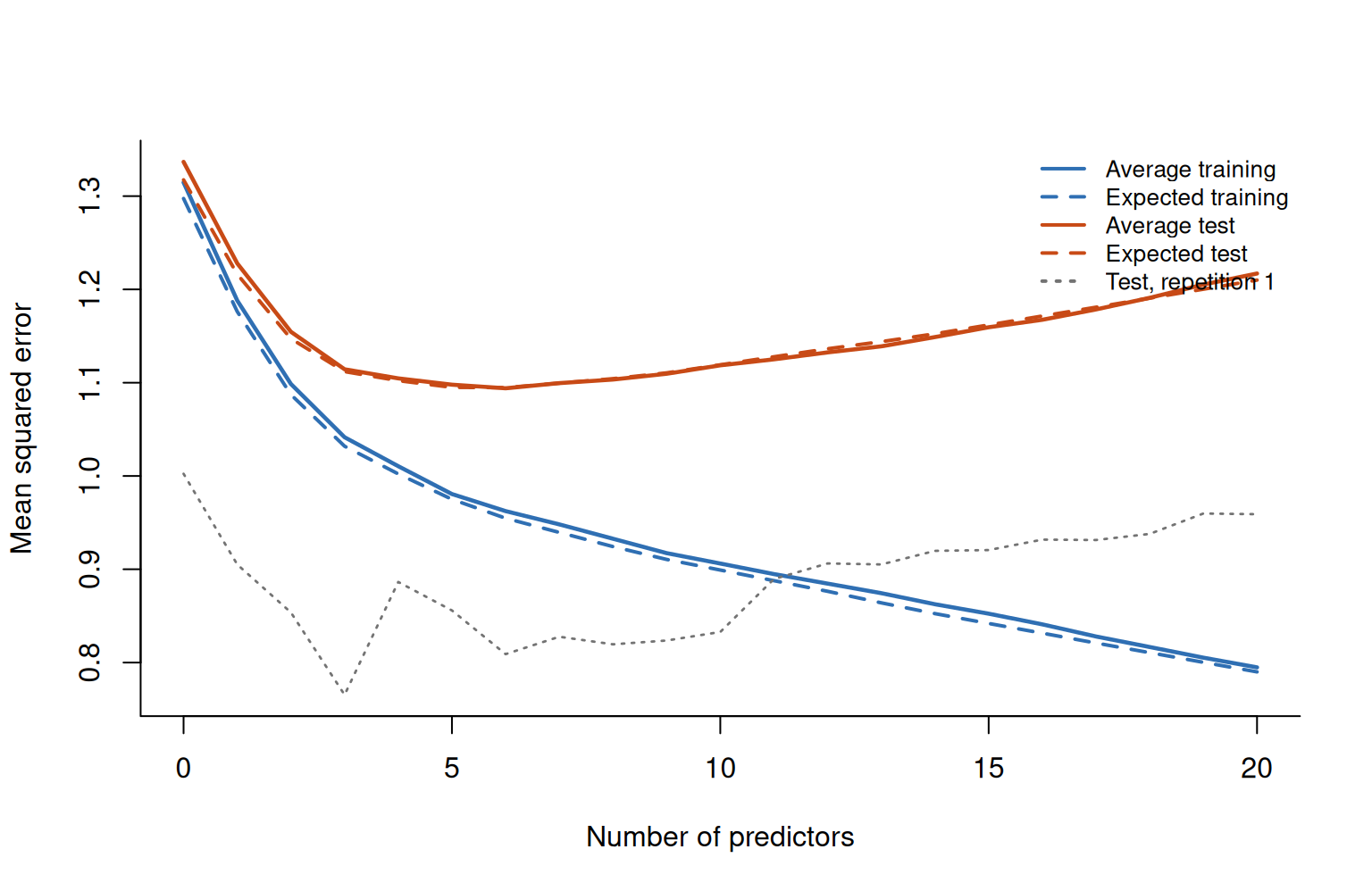
print(results_r[c(1, 6, 11, 16, 21), ], digits = 4)

    m  train theory_train  test theory_test first_test
1   0 1.3147       1.2974 1.337       1.317     1.0024
6   5 0.9806       0.9750 1.098       1.095     0.8559
11 10 0.9061       0.8992 1.119       1.119     0.8328
16 15 0.8524       0.8419 1.159       1.162     0.9206
21 20 0.7948       0.7900 1.217       1.210     0.9590

print(c(training_is_monotone = training_is_monotone))

training_is_monotone 
                TRUE 

print(c(
  minimum_average_test = which.min(results_r$test) - 1,
  minimum_expected_test = which.min(results_r$theory_test) - 1
))

 minimum_average_test minimum_expected_test 
                    6                     6 

matplot(
  results_r$m,
  results_r[c("train", "theory_train", "test", "theory_test", "first_test")],
  type = "l",
  lty = c(1, 2, 1, 2, 3),
  lwd = c(2.3, 2, 2.3, 2, 1.4),
  col = c("#2F6FB3", "#2F6FB3", "#C84A16", "#C84A16", "gray45"),
  xlab = "Number of predictors",
  ylab = "Mean squared error",
  bty = "l"
)
legend(
  "topright",
  legend = c(
    "Average training", "Expected training",
    "Average test", "Expected test", "Test, repetition 1"
  ),
  col = c("#2F6FB3", "#2F6FB3", "#C84A16", "#C84A16", "gray45"),
  lty = c(1, 2, 1, 2, 3),
  lwd = 2,
  bty = "n",
  cex = 0.82
)

Training and test MSE along the nested model sequence.

Python

import numpy as np
import matplotlib.pyplot as plt

rng = np.random.default_rng(43202)
n = 100
p = 20
repetitions = 200

# Generate one covariate matrix, then keep it fixed.
X_all = rng.normal(size=(n, p))
beta = 0.4 ** np.sqrt(np.arange(1, p + 1))
mu = X_all @ beta

# Rows are repetitions; columns are predictor counts 0 through p.
train_mse = np.empty((repetitions, p + 1))
test_mse = np.empty((repetitions, p + 1))

# Each run observes a fresh training and test response.
for k in range(repetitions):
    y_train = mu + rng.normal(size=n)
    y_test = mu + rng.normal(size=n)

    # Compare every candidate model on this same response pair.
    for m in range(p + 1):
        X_m = np.column_stack((np.ones(n), X_all[:, :m]))
        Q = np.linalg.qr(X_m, mode="reduced")[0]
        y_hat = Q @ (Q.T @ y_train)

        train_mse[k, m] = np.mean((y_train - y_hat) ** 2)
        test_mse[k, m] = np.mean((y_test - y_hat) ** 2)

theory_train = np.empty(p + 1)
theory_test = np.empty(p + 1)

# Fit the true mean to calculate the fixed-design approximation bias.
for m in range(p + 1):
    X_m = np.column_stack((np.ones(n), X_all[:, :m]))
    Q = np.linalg.qr(X_m, mode="reduced")[0]
    y_hat = Q @ (Q.T @ mu)
    bias_mse = np.mean((mu - y_hat) ** 2)
    theory_train[m] = bias_mse + 1 - (m + 1) / n
    theory_test[m] = bias_mse + 1 + (m + 1) / n

average_train = train_mse.mean(axis=0)
average_test = test_mse.mean(axis=0)
training_is_monotone = np.all(np.diff(train_mse, axis=1) <= 1e-10)

for m in [0, 5, 10, 15, 20]:
    print(
        f"m={m:2d}, train={average_train[m]:.4f}, "
        f"E(train)={theory_train[m]:.4f}, "
        f"test={average_test[m]:.4f}, "
        f"E(test)={theory_test[m]:.4f}"
    )

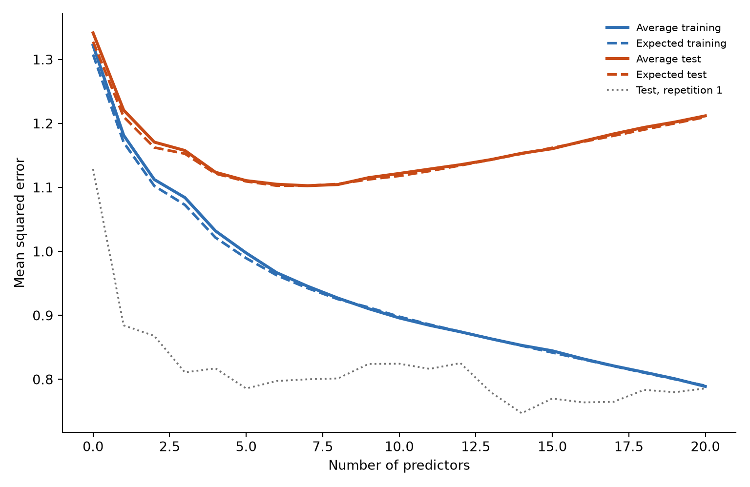
m= 0, train=1.3220, E(train)=1.3078, test=1.3416, E(test)=1.3278
m= 5, train=0.9976, E(train)=0.9894, test=1.1107, E(test)=1.1094
m=10, train=0.8960, E(train)=0.8980, test=1.1218, E(test)=1.1180
m=15, train=0.8446, E(train)=0.8419, test=1.1605, E(test)=1.1619
m=20, train=0.7889, E(train)=0.7900, test=1.2119, E(test)=1.2100

print("Training MSE is monotone:", training_is_monotone)

Training MSE is monotone: True

print("Minimum average test:", int(np.argmin(average_test)))

Minimum average test: 7

print("Minimum expected test:", int(np.argmin(theory_test)))

Minimum expected test: 7

fig, ax = plt.subplots(figsize=(8, 5.2))
m_values = np.arange(p + 1)
ax.plot(m_values, average_train, color="#2F6FB3", lw=2.3,
        label="Average training")
ax.plot(m_values, theory_train, "--", color="#2F6FB3", lw=2,
        label="Expected training")
ax.plot(m_values, average_test, color="#C84A16", lw=2.3,
        label="Average test")
ax.plot(m_values, theory_test, "--", color="#C84A16", lw=2,
        label="Expected test")
ax.plot(m_values, test_mse[0], ":", color="0.45", lw=1.4,
        label="Test, repetition 1")
ax.set(xlabel="Number of predictors", ylabel="Mean squared error")
ax.spines[["top", "right"]].set_visible(False)
ax.legend(frameon=False, fontsize=8)
fig.tight_layout()
plt.show()

Training and test MSE along the nested model sequence.

The simulation averages should be close to their theoretical expectations, apart from Monte Carlo error. The training curve decreases because every larger model contains the previous model.

Expected test MSE contains the mean squared approximation bias $B_m^2/n$, which generally decreases, and the estimation-variance term $(m+1)/n$, which increases. Their competition can produce an interior minimum. A single test-MSE curve is irregular because it retains the random variation from one response vector.

Expected training MSE contains $-(m+1)/n$ instead of $+(m+1)/n$. It therefore rewards the flexibility that allows a model to follow training noise and cannot select the predictor count honestly by itself.

Question 2: Prediction error at one target point

Original question

Let $n=100$, $p=6$, and $\sigma^2=1$. Construct the fixed covariate matrix $\mathbf X_{\mathrm{all}}\in\mathbb R^{n\times p}$ with entries

$$(\mathbf X_{\mathrm{all}})_{ij} =\sqrt{2}\cos\left\{ \frac{\pi j(i-\tfrac12)}{n} \right\}, \qquad i=1,\ldots,n, \quad j=1,\ldots,p.$$

Its columns satisfy

$$\mathbf 1^{\mathsf T}\mathbf X_{\mathrm{all}}=\mathbf 0^{\mathsf T}, \qquad \frac{1}{n}\mathbf X_{\mathrm{all}}^{\mathsf T}\mathbf X_{\mathrm{all}}=\mathbf I_p.$$

Here $\mathbf I_p$ is the $p\times p$ identity matrix.

The following code shows a direct construction of $\mathbf X_{\mathrm{all}}$.

R

n <- 100
p <- 6
X_all <- outer(
  1:n, 1:p,
  function(i, j) sqrt(2) * cos(pi * j * (i - 0.5) / n)
)

Python

import numpy as np

n, p = 100, 6
i = np.arange(1, n + 1)[:, None]
j = np.arange(1, p + 1)[None, :]
X_all = np.sqrt(2) * np.cos(np.pi * j * (i - 0.5) / n)

Keep $\mathbf X_{\mathrm{all}}$ fixed and generate one training response from

$$\mathbf y =\mathbf X_{\mathrm{all}}\boldsymbol\beta+\boldsymbol\epsilon, \qquad \boldsymbol\beta =(0.5,0.5,0.5,0.5,0.5,0.5)^{\mathsf T},$$

where

$$\boldsymbol\epsilon \sim \mathcal N_n(\mathbf 0,\mathbf I_n).$$

Here $\mathbf I_n$ is the $n\times n$ identity matrix.

For $m=0,\ldots,p$, fit a linear model with an intercept and the first $m$ predictors. Consider prediction of the mean response at

$$\mathbf x_0=(0,1,0,0,1,0)^{\mathsf T}.$$

Write

$$\mu_0=\mathbf x_0^{\mathsf T}\boldsymbol\beta,$$

and let $\widehat\mu_{0,m}$ be the prediction from the model containing the first $m$ predictors. Here $x_{0j}$ denotes the $j$th coordinate of $\mathbf x_0$. For this design,

$$E\!\left[ \left(\widehat\mu_{0,m}-\mu_0\right)^2 \mid \mathbf X_{\mathrm{all}} \right] = \left( \sum_{j=m+1}^{p}x_{0j}\beta_j \right)^2 +\frac{\sigma^2}{n} \left( 1+\sum_{j=1}^{m}x_{0j}^2 \right).$$

1. Calculate $\mu_0$, the theoretical squared bias, and the expected squared error for $m=0,\ldots,p$ using the formula above. You do not need to derive the formula. Briefly explain in words why it consists of a squared bias term from omitted predictors and a variance term from estimating coefficients; no proof is required. Identify the values of $m$ where the expected squared error changes and where it remains unchanged.

2. Use seed 43203. Generate the response, fit the models, and calculate

$$\left(\widehat\mu_{0,m}-\mu_0\right)^2.$$

Repeat this independently 200 times. Plot the simulation averages and theoretical expectations together. Report the smallest $m$ that minimizes the theoretical error.

3. All six regression coefficients are nonzero. Explain why only predictors 2 and 5 contribute directly to the mean response at $\mathbf x_0$. Contrast this target-specific error with the test MSE averaged over all rows of $\mathbf X_{\mathrm{all}}$ in Question 1.

Solution

The target mean is

$$\mu_0 =\mathbf x_0^{\mathsf T}\boldsymbol\beta =0.5+0.5 =1.$$

Because the predictor columns are orthogonal, omitting a predictor leaves its contribution to the target mean unexplained. Squaring the combined omitted contribution gives the squared bias term. Estimating the intercept contributes $\sigma^2/n$ to the variance, and each included slope contributes $(\sigma^2/n)x_{0j}^2$. These variances add because the centered, orthogonal columns make the coefficient estimates uncorrelated.

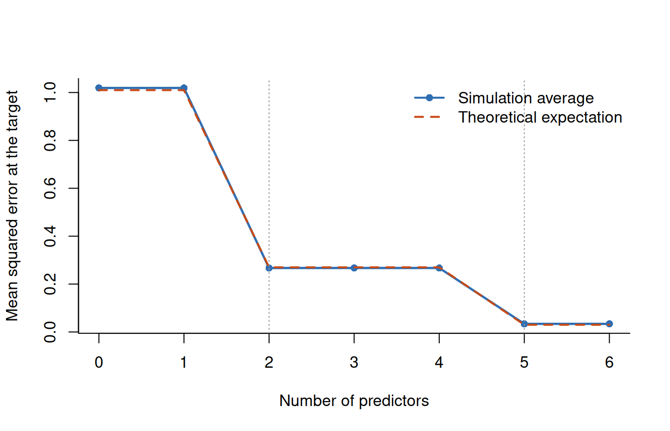
Only coordinates 2 and 5 of $\mathbf x_0$ are nonzero. The theoretical values are:

$m$	Squared target-point bias	Estimation variance	Expected squared error
0	1.00	0.01	1.01
1	1.00	0.01	1.01
2	0.25	0.02	0.27
3	0.25	0.02	0.27
4	0.25	0.02	0.27
5	0.00	0.03	0.03
6	0.00	0.03	0.03

The smallest predictor count that minimizes the expected error is $m=5$.

R

set.seed(43203)
n <- 100
p <- 6
sigma2 <- 1
repetitions <- 200

X_all <- outer(
  1:n, 1:p,
  function(i, j) sqrt(2) * cos(pi * j * (i - 0.5) / n)
)
beta <- rep(0.5, p)
x0 <- c(0, 1, 0, 0, 1, 0)
mu <- drop(X_all %*% beta)
mu0 <- sum(x0 * beta)

stopifnot(
  max(abs(colSums(X_all))) < 1e-10,
  max(abs(crossprod(X_all) / n - diag(p))) < 1e-10
)

# Rows are repetitions; columns are predictor counts 0 through p.
simulation_error <- matrix(NA_real_, repetitions, p + 1)

# Each run observes a fresh response.
for (k in seq_len(repetitions)) {
  y_train <- mu + rnorm(n)

  # Compare every candidate model on this same response.
  for (m in 0:p) {
    X_m <- cbind(1, X_all[, seq_len(m), drop = FALSE])
    beta_hat <- solve(crossprod(X_m), crossprod(X_m, y_train))
    target_row <- c(1, x0[seq_len(m)])
    mu0_hat <- drop(target_row %*% beta_hat)
    simulation_error[k, m + 1] <- (mu0_hat - mu0)^2
  }
}

simulated <- colMeans(simulation_error)
theoretical <- numeric(p + 1)

# Compute the target-specific expectations separately.
for (m in 0:p) {
  omitted <- if (m < p) (m + 1):p else integer(0)
  omitted_signal <- sum(x0[omitted] * beta[omitted])
  estimation_variance <- sigma2 * (1 + sum(x0[seq_len(m)]^2)) / n
  theoretical[m + 1] <- omitted_signal^2 + estimation_variance
}

target_results_r <- data.frame(
  m = 0:p,
  simulated = simulated,
  theoretical = theoretical
)
print(target_results_r, digits = 4)

  m simulated theoretical
1 0   1.01892        1.01
2 1   1.01892        1.01
3 2   0.26712        0.27
4 3   0.26712        0.27
5 4   0.26712        0.27
6 5   0.03376        0.03
7 6   0.03376        0.03

print(c(first_minimum = which.min(theoretical) - 1))

first_minimum 
            5 

plot(
  0:p, simulated,
  type = "o", pch = 16, lwd = 2.3, col = "#2F6FB3",
  xlab = "Number of predictors",
  ylab = "Mean squared error at the target",
  bty = "l"
)
lines(0:p, theoretical, lty = 2, lwd = 2, col = "#C84A16")
abline(v = c(2, 5), lty = 3, col = "gray60")
legend(
  "topright",
  legend = c("Simulation average", "Theoretical expectation"),
  col = c("#2F6FB3", "#C84A16"),
  lty = c(1, 2), pch = c(16, NA), lwd = 2, bty = "n"
)

Squared error at the fixed target point.

Python

import numpy as np
import matplotlib.pyplot as plt

rng_q2 = np.random.default_rng(43203)
n = 100
p = 6
sigma2 = 1.0
repetitions = 200

i = np.arange(1, n + 1)[:, None]
j = np.arange(1, p + 1)[None, :]
X_all = np.sqrt(2) * np.cos(np.pi * j * (i - 0.5) / n)

beta = np.repeat(0.5, p)
x0 = np.array([0, 1, 0, 0, 1, 0], dtype=float)
mu = X_all @ beta
mu0 = x0 @ beta

assert np.allclose(X_all.sum(axis=0), 0, atol=1e-10)
assert np.allclose(X_all.T @ X_all / n, np.eye(p), atol=1e-10)

# Rows are repetitions; columns are predictor counts 0 through p.
simulation_error = np.empty((repetitions, p + 1))

# Each run observes a fresh response.
for k in range(repetitions):
    y_train = mu + rng_q2.normal(size=n)

    # Compare every candidate model on this same response.
    for m in range(p + 1):
        X_m = np.column_stack((np.ones(n), X_all[:, :m]))
        beta_hat = np.linalg.solve(X_m.T @ X_m, X_m.T @ y_train)
        target_row = np.r_[1, x0[:m]]
        mu0_hat = target_row @ beta_hat
        simulation_error[k, m] = (mu0_hat - mu0) ** 2

simulated = simulation_error.mean(axis=0)
theoretical = np.empty(p + 1)

# Compute the target-specific expectations separately.
for m in range(p + 1):
    omitted_signal = x0[m:] @ beta[m:]
    estimation_variance = sigma2 * (1 + x0[:m] @ x0[:m]) / n
    theoretical[m] = omitted_signal**2 + estimation_variance

for m in range(p + 1):
    print(
        f"m={m}, simulated={simulated[m]:.4f}, "
        f"theoretical={theoretical[m]:.4f}"
    )

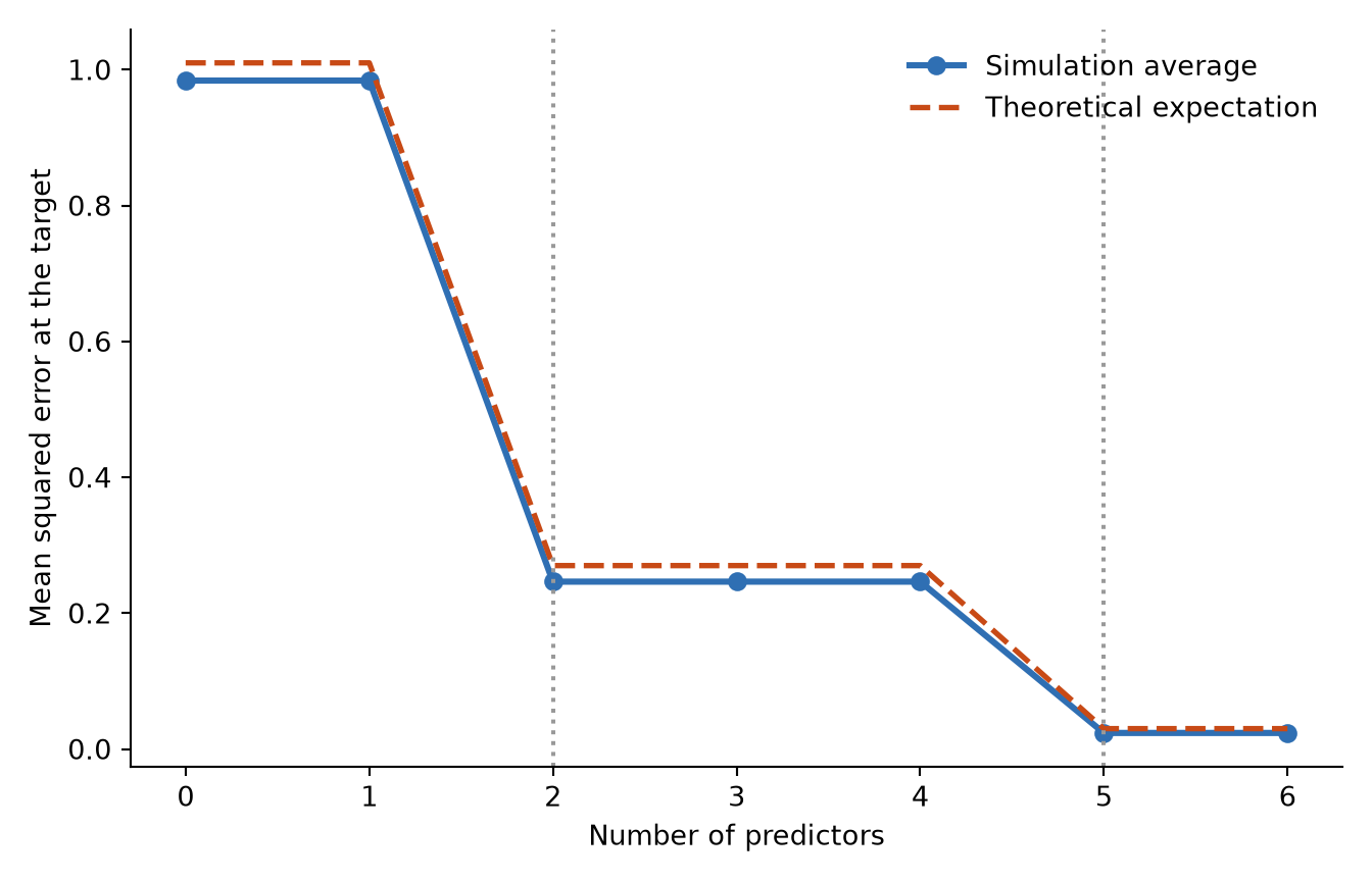
m=0, simulated=0.9839, theoretical=1.0100
m=1, simulated=0.9839, theoretical=1.0100
m=2, simulated=0.2464, theoretical=0.2700
m=3, simulated=0.2464, theoretical=0.2700
m=4, simulated=0.2464, theoretical=0.2700
m=5, simulated=0.0237, theoretical=0.0300
m=6, simulated=0.0237, theoretical=0.0300

print("First minimum:", int(np.argmin(theoretical)))

First minimum: 5

fig, ax = plt.subplots(figsize=(7, 4.5))
m_values = np.arange(p + 1)
ax.plot(m_values, simulated, "o-", color="#2F6FB3", lw=2.3,
        label="Simulation average")
ax.plot(m_values, theoretical, "--", color="#C84A16", lw=2,
        label="Theoretical expectation")
ax.axvline(2, color="0.6", linestyle=":")
ax.axvline(5, color="0.6", linestyle=":")
ax.set(
    xlabel="Number of predictors",
    ylabel="Mean squared error at the target",
    xticks=m_values,
)
ax.spines[["top", "right"]].set_visible(False)
ax.legend(frameon=False)
fig.tight_layout()
plt.show()

Squared error at the fixed target point.

The error changes only when predictor 2 or 5 is added. The other target coordinates are zero, so their fitted coefficients are multiplied by zero in this prediction.

This is a target-specific conclusion. Average test MSE over the entire design gives a predictor weight wherever its values are nonzero across the design rows. A predictor can therefore matter for average prediction even when it does not contribute at one particular target.

Question 3: The optimism correction

Original question

Choose one candidate model before observing the response. Let $p$ be its number of predictors and let $\mathbf X\in\mathbb R^{n\times(p+1)}$ be its full-rank design matrix, including the intercept. The model has $p+1$ fitted coefficients. Let

$$\mathbf H =\mathbf X (\mathbf X^{\mathsf T}\mathbf X)^{-1} \mathbf X^{\mathsf T}$$

be its hat matrix. Suppose

$$\mathbf y=\boldsymbol\mu+\boldsymbol\epsilon, \qquad \mathbf y^*=\boldsymbol\mu+\boldsymbol\epsilon^*,$$

Conditional on the fixed design $\mathbf X$, the two error vectors are independent, have mean zero, and have covariance matrix $\sigma^2\mathbf I_n$. Define

$$\operatorname{MSE}_{\mathrm{train}} = \frac{1}{n} \left\lVert \mathbf y-\mathbf H\mathbf y \right\rVert_2^2, \qquad \operatorname{MSE}_{\mathrm{test}} = \frac{1}{n} \left\lVert \mathbf y^*-\mathbf H\mathbf y \right\rVert_2^2.$$

The conditional bias vector of the fitted mean is

$$E(\mathbf H\mathbf y\mid\mathbf X)-\boldsymbol\mu = -(\mathbf I_n-\mathbf H)\boldsymbol\mu.$$

Let $B^2$ denote the total squared approximation bias:

$$B^2 =\left\lVert (\mathbf I_n-\mathbf H)\boldsymbol\mu \right\rVert_2^2.$$

Thus, $B^2/n$ is the mean squared approximation bias.

You may use

$$\mathbf H^{\mathsf T}=\mathbf H, \qquad \mathbf H^2=\mathbf H, \qquad \operatorname{tr}(\mathbf H)=p+1.$$

For any fixed matrix $\mathbf A$, you may also use

$$E\!\left( \boldsymbol\epsilon^{\mathsf T} \mathbf A \boldsymbol\epsilon \mid \mathbf X \right) =\sigma^2\operatorname{tr}(\mathbf A).$$

1. Derive

$$E(\operatorname{MSE}_{\mathrm{train}}\mid\mathbf X) =\frac{B^2}{n} +\sigma^2\left(1-\frac{p+1}{n}\right),$$

and

$$E(\operatorname{MSE}_{\mathrm{test}}\mid\mathbf X) =\frac{B^2}{n} +\sigma^2\left(1+\frac{p+1}{n}\right).$$

2. Deduce the expected optimism, defined as $E(\operatorname{MSE}_{\mathrm{test}}-\operatorname{MSE}_{\mathrm{train}}\mid\mathbf X)$. For

$$n=120, \qquad p=4, \qquad \frac{B^2}{n}=0.04, \qquad \sigma^2=1,$$

calculate the expected training MSE, expected test MSE, and their difference. Explain why the ordering need not hold for every realized pair of responses.

3. Continue with $n=120$ and $p=4$. Suppose the candidate model has residual sum of squares $\operatorname{RSS}=116.4$, and suppose a common estimate of the error variance is $\widehat\sigma^2=0.96$.

Calculate

$$\widehat{\operatorname{MSE}}_{\mathrm{test}} =\frac{ \operatorname{RSS}+2(p+1)\widehat\sigma^2 }{n},$$

and

$$C_p =\frac{\operatorname{RSS}}{\widehat\sigma^2} -n+2(p+1).$$

Show how these two quantities are related, and explain why minimizing $C_p$ is equivalent to minimizing the corrected test MSE when $n$ and $\widehat\sigma^2$ are common to all candidate models.

Solution

The training residual is

$$\begin{aligned} \mathbf y-\mathbf H\mathbf y &=(\mathbf I_n-\mathbf H) (\boldsymbol\mu+\boldsymbol\epsilon)\\ &=(\mathbf I_n-\mathbf H)\boldsymbol\mu +(\mathbf I_n-\mathbf H)\boldsymbol\epsilon. \end{aligned}$$

The cross term has expectation zero. Since $\mathbf I_n-\mathbf H$ is symmetric and idempotent,

$$\begin{aligned} E\!\left( \left\lVert \mathbf y-\mathbf H\mathbf y \right\rVert_2^2 \mid\mathbf X \right) &= B^2+\sigma^2\operatorname{tr}(\mathbf I_n-\mathbf H)\\ &= B^2+\sigma^2(n-(p+1)). \end{aligned}$$

Dividing by $n$ gives the stated expected training MSE.

For the independent test response,

$$\mathbf y^*-\mathbf H\mathbf y = (\mathbf I_n-\mathbf H)\boldsymbol\mu +\boldsymbol\epsilon^* -\mathbf H\boldsymbol\epsilon.$$

All cross terms again have expectation zero. Independence gives

$$\begin{aligned} E\!\left( \left\lVert \boldsymbol\epsilon^* -\mathbf H\boldsymbol\epsilon \right\rVert_2^2 \mid\mathbf X \right) &= n\sigma^2+ \sigma^2\operatorname{tr}(\mathbf H)\\ &= \sigma^2(n+(p+1)). \end{aligned}$$

Therefore,

$$E(\operatorname{MSE}_{\mathrm{test}}\mid\mathbf X) = \frac{B^2}{n} +\sigma^2\left(1+\frac{p+1}{n}\right).$$

Subtracting the expectations gives

$$E( \operatorname{MSE}_{\mathrm{test}} -\operatorname{MSE}_{\mathrm{train}} \mid\mathbf X ) = \frac{2(p+1)\sigma^2}{n}.$$

For the stated values,

$$E(\operatorname{MSE}_{\mathrm{train}}\mid\mathbf X) = 0.04+1-\frac{4+1}{120} = 0.998333,$$

$$E(\operatorname{MSE}_{\mathrm{test}}\mid\mathbf X) = 0.04+1+\frac{4+1}{120} = 1.081667,$$

and their difference is $0.083333$. These are long-run averages, so a particular test MSE can still be smaller than its corresponding training MSE.

The corrected estimate is

$$\widehat{\operatorname{MSE}}_{\mathrm{test}} = \frac{116.4+2(4+1)(0.96)}{120} = 1.05.$$

Mallows’ $C_p$ is

$$C_p = \frac{116.4}{0.96}-120+2(4+1) = 11.25.$$

Their relationship is

$$\begin{aligned} \frac{\widehat\sigma^2(C_p+n)}{n} &= \frac{0.96(11.25+120)}{120}\\ &= 1.05\\ &= \frac{\operatorname{RSS}+2(p+1)\widehat\sigma^2}{n}. \end{aligned}$$

When $n$ and $\widehat\sigma^2$ are common to all candidates, this is an increasing transformation. The two criteria therefore rank the models in the same order.

Question 4: Comparing Mallows’ $C_p$, AIC, and BIC

Original question

Use data/diabetes.csv, with y as the response. Use rows 1 through 370 as the training data, and let $n=370$ denote the training sample size. Do not use rows 371 through 442 in this question. Fit the following ordinary least-squares models, each with an intercept.

Model	Predictors	$p$
Model A	bmi, bp, s5, sex, s1, s2, s4	7
Model B	all predictors in Model A, followed by s6	8
Full reference	all ten predictors	10

Here $p$ counts predictors, so each model has $p+1$ fitted coefficients including the intercept. Estimate one common noise variance from the full reference model, using $p=10$:

$$\widehat\sigma^2 =\frac{\operatorname{RSS}_{\mathrm{full}}}{n-(p+1)}.$$

For Models A and B, calculate

$$C_p =\frac{\operatorname{RSS}}{\widehat\sigma^2} -n+2(p+1),$$

$$\operatorname{AIC}^{\mathrm{red}} =n\log\left(\frac{\operatorname{RSS}}{n}\right)+2(p+1),$$

and

$$\operatorname{BIC}^{\mathrm{red}} =n\log\left(\frac{\operatorname{RSS}}{n}\right) +(p+1)\log(n).$$

The reduced AIC and BIC omit constants shared by the two candidate models. Smaller values are preferred within each criterion.

1. Fit the three models. Report $p$, RSS, the residual degrees of freedom of the full model, and $\widehat\sigma^2$.

2. Calculate $C_p$, reduced AIC, and reduced BIC for Models A and B. State which model each criterion selects. Do not compare numerical values across different criteria.

3. Compare the improvement in fit from adding s6 with the one-parameter penalty under each criterion. Use this comparison to explain any disagreement. Why does selecting a model not establish that it is the true data-generating model?

Solution

The full model is used only to estimate one common noise variance. Using a different variance estimate for each candidate would change the $C_p$ comparison.

R

data_candidates <- c(
  "data/diabetes.csv",
  "../../../data/week-02/diabetes.csv",
  "data/week-02/diabetes.csv"
)
data_file <- data_candidates[file.exists(data_candidates)][1]
stopifnot(!is.na(data_file))
training <- read.csv(data_file, check.names = FALSE)[1:370, ]
n <- nrow(training)

model_variables <- list(
  A = c("bmi", "bp", "s5", "sex", "s1", "s2", "s4"),
  B = c("bmi", "bp", "s5", "sex", "s1", "s2", "s4", "s6"),
  Full = c(
    "age", "sex", "bmi", "bp", "s1",
    "s2", "s3", "s4", "s5", "s6"
  )
)

fit_rss <- function(variables) {
  # Construct the intercept explicitly so the coefficient count is p + 1.
  X <- cbind(1, as.matrix(training[variables]))
  fit <- lm.fit(X, training$y)
  sum(fit$residuals^2)
}

rss <- vapply(model_variables, fit_rss, numeric(1))
p <- vapply(
  model_variables,
  function(variables) length(variables),
  numeric(1)
)

residual_df <- n - (p["Full"] + 1)
sigma2_hat <- rss["Full"] / residual_df

results_r <- data.frame(
  model = c("Model A", "Model B"),
  p = unname(p[c("A", "B")]),
  rss = unname(rss[c("A", "B")])
)
results_r$cp <- results_r$rss / sigma2_hat - n + 2 * (results_r$p + 1)
results_r$aic <- n * log(results_r$rss / n) + 2 * (results_r$p + 1)
results_r$bic <- n * log(results_r$rss / n) + log(n) * (results_r$p + 1)

fit_gain <- n * log(rss["A"] / rss["B"])
cp_gain <- (rss["A"] - rss["B"]) / sigma2_hat

print(c(residual_df = residual_df, sigma2_hat = sigma2_hat))

residual_df.Full  sigma2_hat.Full 
         359.000         3034.684 

print(results_r, digits = 7)

    model p     rss       cp      aic      bic
1 Model A 7 1098909 8.116253 2974.640 3005.948
2 Model B 8 1089717 7.087434 2973.532 3008.754

print(c(
  aic_bic_fit_gain = fit_gain,
  cp_fit_gain = cp_gain,
  aic_penalty = 2,
  bic_penalty = log(n),
  cp_penalty = 2
))

aic_bic_fit_gain.A      cp_fit_gain.A        aic_penalty        bic_penalty 
          3.107775           3.028819           2.000000           5.913503 
        cp_penalty 
          2.000000 

Python

from pathlib import Path
import numpy as np
import pandas as pd

data_candidates = [
    Path("data/diabetes.csv"),
    Path("../../../data/week-02/diabetes.csv"),
    Path("data/week-02/diabetes.csv"),
]
data_file = next(path for path in data_candidates if path.exists())
training = pd.read_csv(data_file).iloc[:370].copy()
n = len(training)

model_variables = {
    "A": ["bmi", "bp", "s5", "sex", "s1", "s2", "s4"],
    "B": ["bmi", "bp", "s5", "sex", "s1", "s2", "s4", "s6"],
    "Full": [
        "age", "sex", "bmi", "bp", "s1",
        "s2", "s3", "s4", "s5", "s6",
    ],
}


def fit_rss(variables):
    # Construct the intercept explicitly so the coefficient count is p + 1.
    X = np.column_stack((
        np.ones(n),
        training[variables].to_numpy(),
    ))
    beta_hat = np.linalg.lstsq(
        X, training["y"].to_numpy(), rcond=None
    )[0]
    residuals = training["y"].to_numpy() - X @ beta_hat
    return float(residuals @ residuals)


rss = {
    name: fit_rss(variables)
    for name, variables in model_variables.items()
}
p = {
    name: len(variables)
    for name, variables in model_variables.items()
}

residual_df = n - (p["Full"] + 1)
sigma2_hat = rss["Full"] / residual_df

results_py = pd.DataFrame({
    "model": ["Model A", "Model B"],
    "p": [p["A"], p["B"]],
    "rss": [rss["A"], rss["B"]],
})
results_py["cp"] = (
    results_py["rss"] / sigma2_hat - n + 2 * (results_py["p"] + 1)
)
results_py["aic"] = (
    n * np.log(results_py["rss"] / n) + 2 * (results_py["p"] + 1)
)
results_py["bic"] = (
    n * np.log(results_py["rss"] / n) + np.log(n) * (results_py["p"] + 1)
)

fit_gain = n * np.log(rss["A"] / rss["B"])
cp_gain = (rss["A"] - rss["B"]) / sigma2_hat

print({"residual_df": residual_df, "sigma2_hat": sigma2_hat})

{'residual_df': 359, 'sigma2_hat': 3034.684460220173}

print(results_py.round(6).to_string(index=False))

  model  p          rss       cp         aic         bic
Model A  7 1.098909e+06 8.116253 2974.640260 3005.948284
Model B  8 1.089717e+06 7.087434 2973.532485 3008.754012

print({
    "aic_bic_fit_gain": fit_gain,
    "cp_fit_gain": cp_gain,
    "aic_penalty": 2,
    "bic_penalty": np.log(n),
    "cp_penalty": 2,
})

{'aic_bic_fit_gain': np.float64(3.1077752483644665), 'cp_fit_gain': 3.028818636880371, 'aic_penalty': 2, 'bic_penalty': np.float64(5.91350300563827), 'cp_penalty': 2}

The full model has

$$n-(10+1)=359$$

residual degrees of freedom. Therefore,

$$\widehat\sigma^2 =3034.684460.$$

The candidate results are:

Model	$p$	RSS	$C_p$	Reduced AIC	Reduced BIC
Model A	7	1,098,908.566	8.116	2,974.640	3,005.948
Model B	8	1,089,717.057	7.087	2,973.532	3,008.754

Mallows’ $C_p$ and AIC select Model B, while BIC selects Model A. The improvement in the AIC and BIC fit term is

$$n\log\left( \frac{\operatorname{RSS}_{A}} {\operatorname{RSS}_{B}} \right) =3.108.$$

This exceeds AIC’s additional penalty of $2$, but is smaller than BIC’s additional penalty $\log(n)=5.914$. On the $C_p$ scale,

$$\frac{ \operatorname{RSS}_{A}-\operatorname{RSS}_{B} }{ \widehat\sigma^2 } =3.029>2.$$

Thus, AIC and $C_p$ accept the improvement from adding s6, while BIC does not. This is a comparison of two candidates under particular assumptions. It does not prove that either candidate is the true data-generating model.

Question 5: Validation and final test data

Original question

Use rows 1 through 370 of diabetes.csv as the training data and rows 371 through 442 as the final test data. Consider eleven nested candidate models. For $m=0,1,\ldots,10$, the model with $m$ predictors contains an intercept and the first $m$ predictors in this order:

age, sex, bmi, bp, s1, s2, s3, s4, s5, s6.

An analyst proposes the following procedure:

1. Fit all eleven candidate models using the training data.
2. Calculate the MSE of each model on the final test data.
3. Select the model with the smallest test MSE.
4. Report that minimum as the final estimate of prediction error.

The analyst argues that the procedure is valid because the final test data were not used to estimate the regression coefficients.

1. Identify the first step that misuses the final test data. Explain why the minimum of eleven test MSE values is generally too favorable as an estimate of the selected procedure’s future prediction error.

2. Rewrite the analysis using five-fold cross-validation within the training data. State how the predictor count is selected, what is refitted, and when the final test data may be used.

3. Suppose the analyst has already examined all eleven test MSE values. What can still be reported transparently, and what additional data would be needed for a new final evaluation?

Solution

Step 2 is the first misuse. The final test responses are used to compare the candidates, so predictor count is selected using the final test data even though the coefficients were fitted using only the training data.

Each test MSE contains random variation. Taking the minimum tends to select a model whose test MSE was unusually small by chance. Reporting the same minimum as the final assessment therefore gives an optimistic estimate of future prediction error.

A valid procedure is:

1. Reserve rows 371 through 442 without inspecting their responses.
2. Divide rows 1 through 370 into five folds.
3. For each predictor count, fit on four folds and calculate MSE on the remaining fold. Repeat until every fold has served once as the validation fold.
4. Average the five validation MSE values and select the predictor count with the smallest average.
5. Refit the selected model using all 370 training observations.
6. Evaluate this fitted model once on rows 371 through 442.

Any data-dependent preprocessing must also be estimated within the four training folds. If all eleven final test MSE values have already been examined, the analysis can still be reported as exploratory, but the reported minimum is not an untouched final assessment. A new independent test dataset or genuinely future observations are needed for a new final evaluation.

Key ideas

1. Under a fixed design, training and test responses differ only through independent response noise.
2. Average prediction error and prediction error at one target point can favor different predictor counts.
3. The fixed-design optimism correction is $2(p+1)\sigma^2/n$.
4. Mallows’ $C_p$, AIC, and BIC can disagree because they use different complexity penalties.
5. A final test set is valid only if it remains untouched until the entire procedure has been chosen.

Reference

James, Witten, Hastie, Tibshirani, and Taylor, An Introduction to Statistical Learning, Chapters 3, 5, and 6.