Skip to main content

Homework 01 Solutions

On this page

• Before you begin
• Question 1 (Least squares and matrix calculations)
• Question 2 (Gaussian likelihood for linear regression)
• Question 3 (Starting values in nonconvex optimization)
• Question 4 (Nearly collinear predictors)
• Question 5 (Data preparation and summary statistics)
• Question 6 (Can 39 million Fitbit records represent US adults?)

Before you begin

Each section repeats the original question before giving the solution. Complete all six questions and compare your reasoning with the explanation before opening the code. Questions 1 through 5 have comparable R and Python solutions, but you need to work in only one language.

The simulations in Questions 1, 2, and 4 are generated directly in each language. R and NumPy use different random-number generators, so the same seed does not produce identical observations across the two languages. Each analysis is reproducible within its language, and the statistical model, algebraic identities, and interpretations agree. Only Question 5 uses a supplied data file.

Download the materials

• Download solutions-01.qmd
• Download homework-01.qmd
• Download combined ZIP file

Extract the ZIP file inside the homework/ folder of your stat432-fall2026 repository. It creates week-01/, so the complete path is homework/week-01/. The folder contains the editable homework and solution files, together with the data file used in Question 5.

Question 1 (Least squares and matrix calculations)

Original question

Set the random seed to 43201. Generate $n=100$ observations with $p=5$ predictors according to

$$x_{ij}\overset{\mathrm{iid}}{\sim}N(0,1), \qquad \varepsilon_i\overset{\mathrm{iid}}{\sim}N(0,0.7^2),$$

with all predictors and errors generated independently. Let

$$\mathbf X = \begin{bmatrix} \mathbf 1 & \mathbf x_1 & \cdots & \mathbf x_5 \end{bmatrix}, \qquad \boldsymbol\beta = (3,1.4,-0.9,0.7,0,1.1)^{\mathsf T},$$

and generate

$$\mathbf y=\mathbf X\boldsymbol\beta+\boldsymbol\varepsilon.$$

1. Generate the data and report the dimensions and rank of $\mathbf X$. Calculate the least-squares estimate $\widehat{\boldsymbol\beta}$ using a numerically stable least-squares routine, without explicitly calculating $(\mathbf X^{\mathsf T}\mathbf X)^{-1}$. Compare the estimates with the coefficients used to generate the data.

2. Calculate the fitted values, the residual vector $\mathbf r=\mathbf y-\mathbf X\widehat{\boldsymbol\beta}$, and the training root mean squared error

$$\operatorname{RMSE} = \left( \frac{1}{n}\sum_{i=1}^{n}r_i^2 \right)^{1/2}.$$

3. Report $\lVert\mathbf X^{\mathsf T}\mathbf r\rVert_\infty$. Explain why this value should be close to zero and what it tells us about the residual vector.

Solution

The coefficient vector used to generate the response is

$$\boldsymbol\beta = (3,1.4,-0.9,0.7,0,1.1)^{\mathsf T}.$$

The first column of (X) is the intercept column. The other five columns contain the simulated predictors, so (X) has (100) rows and (6) columns. With probability one, a Gaussian design of this size has full column rank. The generated design has rank (6) in both implementations.

For a full-rank design, the least-squares estimate is the unique minimizer of

$$L(\boldsymbol\beta) = \lVert\mathbf y-\mathbf X\boldsymbol\beta\rVert_2^2.$$

A stable least-squares routine based on a QR or singular-value decomposition should be used. Forming ((X^{T}X)^{-1}) explicitly is unnecessary and can amplify numerical error.

The fitted values and residuals are

$$\widehat{\mathbf y} = \mathbf X\widehat{\boldsymbol\beta}, \qquad \mathbf r = \mathbf y-\widehat{\mathbf y}.$$

The estimates will not equal the generating coefficients exactly because this exercise uses one realization of the noise. The R estimates are approximately

$$(3.006,\ 1.417,\ -0.888,\ 0.795,\ 0.048,\ 1.132)^{\mathsf T},$$

while the Python estimates are approximately

$$(2.973,\ 1.324,\ -0.841,\ 0.720,\ -0.083,\ 1.165)^{\mathsf T}.$$

Both sets are reasonably close to the generating values. In particular, the estimated coefficient of (x_4) is near its true value of zero.

Differentiating the least-squares objective gives

$$\nabla L(\boldsymbol\beta) = -2\mathbf X^{\mathsf T} (\mathbf y-\mathbf X\boldsymbol\beta).$$

At the minimizer,

$$\mathbf X^{\mathsf T}\mathbf r \approx \mathbf 0.$$

The approximation accounts only for floating-point arithmetic. Geometrically, the residual vector is orthogonal to every column of (X), including the intercept column. The latter also implies that the residuals sum to approximately zero.

R

set.seed(43201)

n <- 100
p <- 5

# Generate the predictors and name the columns to match the notation.
x <- matrix(rnorm(n * p), nrow = n, ncol = p)
colnames(x) <- paste0("x", seq_len(p))

X <- cbind("(Intercept)" = 1, x)
beta <- c(
  "(Intercept)" = 3,
  x1 = 1.4,
  x2 = -0.9,
  x3 = 0.7,
  x4 = 0,
  x5 = 1.1
)

epsilon <- rnorm(n, mean = 0, sd = 0.7)
y <- as.vector(X %*% beta + epsilon)

# lm.fit uses a stable QR-based least-squares calculation.
least_squares_fit <- lm.fit(x = X, y = y)
beta_hat <- least_squares_fit$coefficients
fitted_values <- as.vector(X %*% beta_hat)
residuals <- y - fitted_values

coefficient_comparison <- data.frame(
  coefficient = names(beta),
  truth = unname(beta),
  estimate = unname(beta_hat)
)

training_rmse <- sqrt(mean(residuals^2))
normal_equation_error <- max(abs(crossprod(X, residuals)))

print(dim(X))
print(qr(X)$rank)
print(coefficient_comparison)
print(training_rmse)
print(normal_equation_error)

[1] 100   6
[1] 6
  coefficient truth   estimate
1 (Intercept)   3.0  3.0063210
2          x1   1.4  1.4171604
3          x2  -0.9 -0.8883453
4          x3   0.7  0.7952834
5          x4   0.0  0.0484378
6          x5   1.1  1.1319341
[1] 0.6763696
[1] 1.909584e-14

The training RMSE is approximately (0.6764), and (X^{T}r_) is about (5.9^{-14}).

Python

import numpy as np

rng = np.random.default_rng(43201)

n = 100
p = 5

# Generate the five predictors and add the intercept column.
x = rng.normal(size=(n, p))
X = np.column_stack([np.ones(n), x])
beta = np.array([3.0, 1.4, -0.9, 0.7, 0.0, 1.1])

epsilon = rng.normal(loc=0.0, scale=0.7, size=n)
y = X @ beta + epsilon

# lstsq uses a stable singular-value-based calculation.
beta_hat, _, rank, _ = np.linalg.lstsq(X, y, rcond=None)
fitted_values = X @ beta_hat
residuals = y - fitted_values

coefficient_comparison = np.column_stack([beta, beta_hat])
training_rmse = np.sqrt(np.mean(residuals**2))
normal_equation_error = np.max(np.abs(X.T @ residuals))

print("Dimensions:", X.shape)
print("Rank:", rank)
print("Truth and estimate:")
print(coefficient_comparison)
print("Training RMSE:", training_rmse)
print("Normal-equation error:", normal_equation_error)

Dimensions: (100, 6)
Rank: 6
Truth and estimate:
[[ 3.          2.97306594]
 [ 1.4         1.32402032]
 [-0.9        -0.84148921]
 [ 0.7         0.7204349 ]
 [ 0.         -0.08314353]
 [ 1.1         1.16505507]]
Training RMSE: 0.6463397227026199
Normal-equation error: 1.2827533168746823e-12

The training RMSE is approximately (0.6463), and (X^{T}r_) is about (1.4^{-12}).

Question 2 (Gaussian likelihood for linear regression)

Original question

Continue with the data from Question 1. Suppose

$$\mathbf Y\mid\mathbf X \sim N_n\left(\mathbf X\boldsymbol\beta,\sigma^2\mathbf I_n\right).$$

The log-likelihood, including the constant term, is

$$\ell(\boldsymbol\beta,\sigma^2) = -\frac{n}{2}\log(2\pi\sigma^2) -\frac{1}{2\sigma^2} (\mathbf y-\mathbf X\boldsymbol\beta)^{\mathsf T} (\mathbf y-\mathbf X\boldsymbol\beta).$$

1. For fixed $\sigma^2$, explain why maximizing $\ell(\boldsymbol\beta,\sigma^2)$ over $\boldsymbol\beta$ is equivalent to minimizing the residual sum of squares. What does this imply about the maximum-likelihood estimate of $\boldsymbol\beta$?

2. For fixed $\boldsymbol\beta$, differentiate the log-likelihood with respect to $\sigma^2$ and derive its maximum-likelihood estimate. Calculate this estimate at $\widehat{\boldsymbol\beta}$ and compare it with the unbiased estimate of $\sigma^2$. Explain why the two denominators differ.

3. Let

$$\mathbf e_{x_2}=(0,0,1,0,0,0)^{\mathsf T}.$$

Using the variance estimate from part b, plot

$$\ell\left( \widehat{\boldsymbol\beta}+t\mathbf e_{x_2}, \widehat{\sigma}_{\mathrm{MLE}}^2 \right)$$

over a grid of $t$ values from $-1.25$ to $1.25$. State where the maximum occurs and explain why this agrees with the least-squares result.

Solution

For fixed (^2), the first term in the log-likelihood does not depend on (), and the multiplier of the residual sum of squares is negative. Therefore,

$$\underset{\boldsymbol\beta}{\operatorname{argmax}}\, \ell(\boldsymbol\beta,\sigma^2) = \underset{\boldsymbol\beta}{\operatorname{argmin}}\, \lVert\mathbf y-\mathbf X\boldsymbol\beta\rVert_2^2.$$

Thus, the maximum-likelihood estimate of () is the least-squares estimate from Question 1.

To optimize with respect to the variance, write (v=^2) and hold () fixed. If

$$\operatorname{RSS}(\boldsymbol\beta) = \lVert\mathbf y-\mathbf X\boldsymbol\beta\rVert_2^2,$$

then

$$\ell(\boldsymbol\beta,v) = -\frac{n}{2}\log(2\pi v) -\frac{\operatorname{RSS}(\boldsymbol\beta)}{2v}.$$

Its derivative is

$$\frac{\partial\ell}{\partial v} = -\frac{n}{2v} + \frac{\operatorname{RSS}(\boldsymbol\beta)}{2v^2}.$$

Setting the derivative equal to zero gives

$$\widehat{\sigma}_{\mathrm{MLE}}^2 = \widehat v = \frac{\operatorname{RSS}}{n}.$$

At this value, the second derivative is (-n/(2v^2)<0), so the stationary point is a maximum.

The usual unbiased estimator is

$$\widehat{\sigma}_{\mathrm{unbiased}}^2 = \frac{\operatorname{RSS}}{n-6}.$$

The maximum-likelihood calculation divides by (n) because it directly maximizes the likelihood. The unbiased calculation divides by (n-6) because six regression coefficients were estimated. Under the Gaussian linear model,

$$\mathbb E(\operatorname{RSS}) = (n-6)\sigma^2.$$

The R estimates are approximately (0.4575) and (0.4867), while the Python estimates are approximately (0.4178) and (0.4444), for the maximum-likelihood and unbiased versions, respectively.

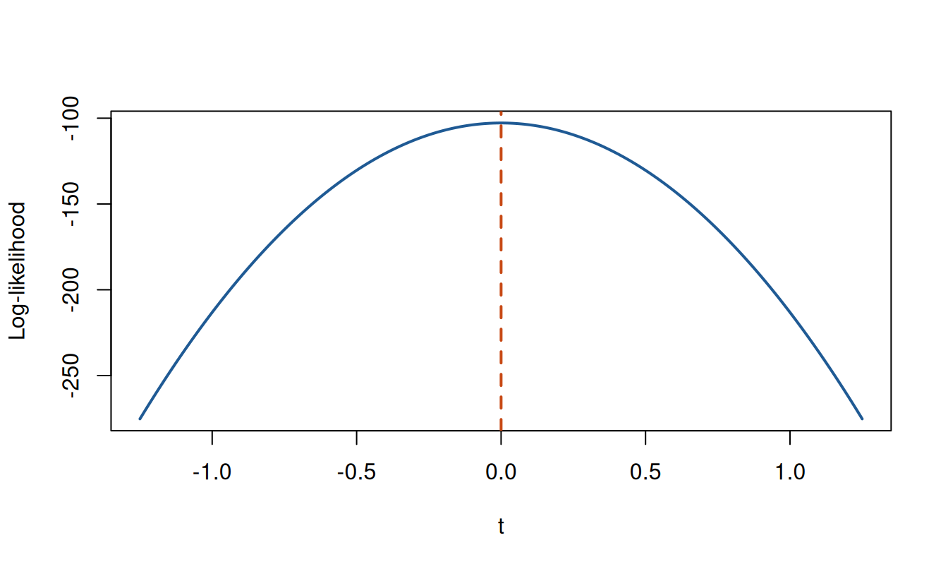
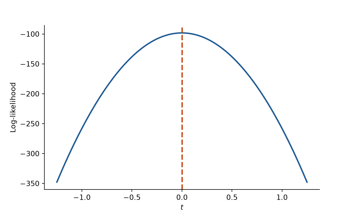
For the likelihood profile, (t=0) corresponds to (). Moving away from zero changes only the coefficient of (x_2), increases the residual sum of squares, and decreases the log-likelihood. The maximum therefore occurs at (t=0), as the plot confirms.

R

rss <- sum(residuals^2)
sigma2_mle <- rss / n
sigma2_unbiased <- rss / (n - ncol(X))

log_likelihood <- function(beta_value, sigma2, X, y) {
  residual <- y - as.vector(X %*% beta_value)
  -nrow(X) / 2 * log(2 * pi * sigma2) -
    sum(residual^2) / (2 * sigma2)
}

e_x2 <- c(0, 0, 1, 0, 0, 0)
t_grid <- seq(-1.25, 1.25, length.out = 251)
profile_log_likelihood <- vapply(
  t_grid,
  function(t) {
    log_likelihood(
      beta_hat + t * e_x2,
      sigma2_mle,
      X,
      y
    )
  },
  numeric(1)
)

print(c(
  sigma2_mle = sigma2_mle,
  sigma2_unbiased = sigma2_unbiased,
  maximizing_t = t_grid[which.max(profile_log_likelihood)]
))

plot(
  t_grid,
  profile_log_likelihood,
  type = "l",
  lwd = 2,
  col = "#1F5A94",
  xlab = expression(t),
  ylab = "Log-likelihood"
)
abline(v = 0, lty = 2, lwd = 2, col = "#C84A16")

Likelihood profile for the coefficient of x2.

     sigma2_mle sigma2_unbiased    maximizing_t 
      0.4574759       0.4866765       0.0000000 

Python

import matplotlib.pyplot as plt

rss = residuals @ residuals
sigma2_mle = rss / n
sigma2_unbiased = rss / (n - X.shape[1])

def log_likelihood(beta_value, sigma2, X, y):
    residual = y - X @ beta_value
    return (
        -X.shape[0] / 2 * np.log(2 * np.pi * sigma2)
        - residual @ residual / (2 * sigma2)
    )

e_x2 = np.array([0.0, 0.0, 1.0, 0.0, 0.0, 0.0])
t_grid = np.linspace(-1.25, 1.25, 251)
profile_log_likelihood = np.array(
    [
        log_likelihood(
            beta_hat + t * e_x2,
            sigma2_mle,
            X,
            y,
        )
        for t in t_grid
    ]
)

print("MLE variance:", sigma2_mle)
print("Unbiased variance:", sigma2_unbiased)
print("Maximizing t:", t_grid[np.argmax(profile_log_likelihood)])

fig, ax = plt.subplots(figsize=(7, 4.2))
profile_line = ax.plot(
    t_grid,
    profile_log_likelihood,
    color="#1F5A94",
    linewidth=2,
)
zero_line = ax.axvline(
    0,
    color="#C84A16",
    linestyle="--",
    linewidth=2,
)
profile_labels = ax.set(xlabel=r"$t$", ylabel="Log-likelihood")
ax.spines[["top", "right"]].set_visible(False)
plt.show()

MLE variance: 0.4177550371432995
Unbiased variance: 0.44442025228010584
Maximizing t: 0.0

Likelihood profile for the coefficient of x2.

Question 3 (Starting values in nonconvex optimization)

Original question

Consider the function

$$f(x)=\exp(1.5x)-3(x+6)^2-0.05x^3,$$

with derivative

$$f'(x)=1.5\exp(1.5x)-6(x+6)-0.15x^2.$$

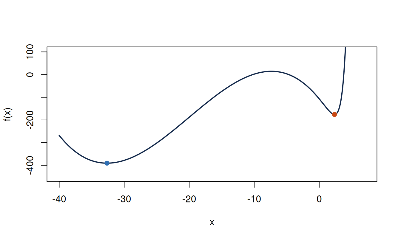
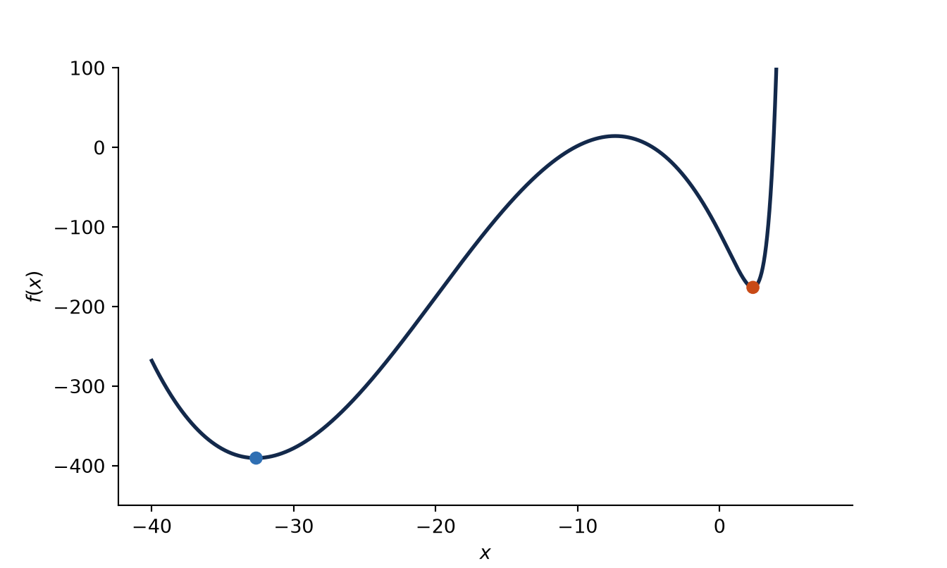
1. Plot $f(x)$ over the interval $[-40,7]$. Based on the plot, describe the important features of the objective function that may affect numerical optimization.

2. Use BFGS to minimize $f(x)$ twice, starting at $x^{(0)}=-15$ and $x^{(0)}=0$. Supply $f'(x)$ to the optimizer. For each run, report the final value of $x$, the final objective value, $|f'(x)|$, and whether the optimizer reported convergence.

3. Explain why the two runs can converge to different answers. Which run gives the lower objective value? What additional evidence would be needed before claiming that this point is the global minimum?

Solution

The objective rises sharply near the right side of the interval. To keep both low regions visible, the figure below displays the vertical range from (-450) to (100); this changes only the display, not the function used by the optimizer. The focused view shows two local minima separated by a local maximum. A gradient-based optimizer uses local information, so its path depends on the starting point and on which basin of attraction contains that point.

Starting from (-15), both implementations converge to approximately

$$x=-32.64911, \qquad f(x)=-390.38577.$$

Starting from (0), they converge to approximately

$$x=2.34997, \qquad f(x)=-175.86262.$$

The reported gradients are close to zero, and both optimizers report convergence. These facts show that each run found a stationary local minimum. They do not show that both runs found the same minimum or that either result is globally optimal.

The run starting at (-15) gives the lower objective value. Before claiming a global minimum, we would need evidence that no lower region was missed. For this one-dimensional problem, a strong argument could combine the limiting behavior of (f(x)) as (x-) and (x+), a search for all roots of (f’(x)), and a comparison of (f(x)) at every stationary point. A dense plot or many starting values provide useful numerical evidence, but by themselves they do not prove global optimality.

R

objective <- function(x) {
  exp(1.5 * x) - 3 * (x + 6)^2 - 0.05 * x^3
}

gradient <- function(x) {
  1.5 * exp(1.5 * x) - 6 * (x + 6) - 0.15 * x^2
}

x_grid <- seq(-40, 7, length.out = 1200)

# Restrict only the displayed vertical range so both minima are visible.
plot(
  x_grid,
  objective(x_grid),
  type = "l",
  lwd = 2,
  col = "#13294B",
  ylim = c(-450, 100),
  xlab = "x",
  ylab = "f(x)"
)

starts <- c(-15, 0)
optimization_results <- lapply(
  starts,
  function(start) {
    optim(
      par = start,
      fn = objective,
      gr = gradient,
      method = "BFGS"
    )
  }
)

optimization_summary <- do.call(
  rbind,
  Map(
    function(start, result) {
      data.frame(
        starting_value = start,
        final_x = result$par,
        objective = result$value,
        absolute_gradient = abs(gradient(result$par)),
        converged = result$convergence == 0
      )
    },
    starts,
    optimization_results
  )
)

points(
  optimization_summary$final_x,
  optimization_summary$objective,
  pch = 19,
  col = c("#2F6FB3", "#C84A16")
)

Nonconvex objective and the two BFGS solutions.

print(optimization_summary)

  starting_value    final_x objective absolute_gradient converged
1            -15 -32.649111 -390.3858      8.725087e-08      TRUE
2              0   2.349967 -175.8626      6.556057e-07      TRUE

Python

from scipy.optimize import minimize

def objective(x):
    return np.exp(1.5 * x) - 3 * (x + 6) ** 2 - 0.05 * x**3

def gradient(x):
    return 1.5 * np.exp(1.5 * x) - 6 * (x + 6) - 0.15 * x**2

x_grid = np.linspace(-40, 7, 1200)

fig, ax = plt.subplots(figsize=(7, 4.2))
objective_line = ax.plot(
    x_grid,
    objective(x_grid),
    color="#13294B",
    linewidth=2,
)
objective_labels = ax.set(
    ylim=(-450, 100),
    xlabel=r"$x$",
    ylabel=r"$f(x)$",
)
ax.spines[["top", "right"]].set_visible(False)

starts = [-15.0, 0.0]
optimization_results = []
for start in starts:
    result = minimize(
        fun=lambda value: objective(value[0]),
        x0=np.array([start]),
        jac=lambda value: np.array([gradient(value[0])]),
        method="BFGS",
    )
    optimization_results.append(result)

optimization_summary = []
for start, result in zip(starts, optimization_results):
    optimization_summary.append(
        {
            "starting_value": start,
            "final_x": result.x[0],
            "objective": result.fun,
            "absolute_gradient": abs(gradient(result.x[0])),
            "converged": result.success,
        }
    )

minimum_points = ax.scatter(
    [result.x[0] for result in optimization_results],
    [result.fun for result in optimization_results],
    color=["#2F6FB3", "#C84A16"],
    zorder=3,
)
plt.show()

for row in optimization_summary:
    print(
        f"start={row['starting_value']:5.1f}, "
        f"x={float(row['final_x']): .6f}, "
        f"f(x)={float(row['objective']): .6f}, "
        f"|f'(x)|={float(row['absolute_gradient']):.3e}, "
        f"converged={row['converged']}"
    )

Nonconvex objective and the two BFGS solutions.

start=-15.0, x=-32.649111, f(x)=-390.385770, |f'(x)|=2.842e-14, converged=True
start=  0.0, x= 2.349967, f(x)=-175.862620, |f'(x)|=8.127e-06, converged=True

Question 4 (Nearly collinear predictors)

Original question

Continue with $\mathbf X$ and $\mathbf y$ from Question 1. Set the random seed to 43202 and generate

$$u_i\overset{\mathrm{iid}}{\sim}N(0,1), \qquad i=1,\ldots,n.$$

Define

$$\mathbf x_6=\mathbf x_1+10^{-4}\mathbf u, \qquad \mathbf X_+ = \begin{bmatrix} \mathbf X & \mathbf x_6 \end{bmatrix},$$

and let

$$\mathbf y^\star=\mathbf y+10^{-3}\mathbf u.$$

Use a numerically stable least-squares routine throughout.

1. Fit $\mathbf y$ using $\mathbf X$ and $\mathbf X_+$. For each design matrix, report the condition number and training RMSE. For the augmented fit, also report the coefficients of $\mathbf x_1$ and $\mathbf x_6$.

2. Fit $\mathbf y^\star$ using $\mathbf X_+$. Report the changes in the coefficients of $\mathbf x_1$ and $\mathbf x_6$. Compare the two fitted-value vectors using their root mean squared difference and maximum absolute difference.

3. Use the identity

$$\mathbf y^\star-\mathbf y = 10(\mathbf x_6-\mathbf x_1)$$

to explain why the fitted values change very little while the two coefficients change substantially. What does this example suggest about interpreting separate effects for nearly collinear predictors?

Solution

The original design is well conditioned, but the augmented design is not. Since

$$\mathbf x_6-\mathbf x_1 = 10^{-4}\mathbf u,$$

the two columns differ only in a very small direction. The augmented design therefore contains a direction in coefficient space that changes the fitted values very little.

With the stated seeds, the condition number increases from about (1.5) to about (2^4) in both languages. The training RMSE changes only slightly. The separate coefficients of (x_1) and (x_6), however, become very large with opposite signs:

Implementation	(_1)	(_6)	(_1+_6)
R	351.677	-350.259	1.418
Python	-1329.743	1331.060	1.317

The signs and magnitudes differ because the two languages generate different realizations of (u). The important pattern is the same. The individual coefficients are unstable, while their sum remains near the coefficient of (x_1) from the original fit.

The response perturbation satisfies

$$\begin{aligned} \mathbf y^\star-\mathbf y &= 10^{-3}\mathbf u\\ &= 10^{-3} \frac{\mathbf x_6-\mathbf x_1}{10^{-4}}\\ &= 10(\mathbf x_6-\mathbf x_1). \end{aligned}$$

Consequently, the augmented fit can reproduce the response change by changing the two coefficients according to

$$\Delta\widehat\beta_1=-10, \qquad \Delta\widehat\beta_6=10,$$

with all other coefficient changes equal to zero, apart from floating-point error. The corresponding fitted-value change is only (10^{-3}u), whose entries are typically around one-thousandth.

The root mean squared fitted-value difference is approximately (0.00102) in R and (0.000975) in Python. The maximum absolute difference is approximately (0.00257) in R and (0.00235) in Python. Thus, large changes in separate coefficients do not imply large changes in predictions. When predictors are nearly collinear, the data identify their combined contribution much more clearly than their separate effects.

R

set.seed(43202)
u <- rnorm(n)

x6 <- x[, "x1"] + 1e-4 * u
X_plus <- cbind(X, x6 = x6)
y_star <- y + 1e-3 * u

fit_original <- lm.fit(x = X, y = y)
fit_augmented <- lm.fit(x = X_plus, y = y)
fit_perturbed <- lm.fit(x = X_plus, y = y_star)

beta_augmented <- fit_augmented$coefficients
beta_perturbed <- fit_perturbed$coefficients

fitted_augmented <- as.vector(X_plus %*% beta_augmented)
fitted_perturbed <- as.vector(X_plus %*% beta_perturbed)

condition_number <- function(design) {
  singular_values <- svd(design, nu = 0, nv = 0)$d
  max(singular_values) / min(singular_values)
}

fit_summary <- data.frame(
  design = c("X", "X_plus"),
  condition_number = c(
    condition_number(X),
    condition_number(X_plus)
  ),
  training_rmse = c(
    sqrt(mean(fit_original$residuals^2)),
    sqrt(mean(fit_augmented$residuals^2))
  )
)

coefficient_summary <- data.frame(
  response = c("y", "y_star"),
  beta_x1 = c(beta_augmented["x1"], beta_perturbed["x1"]),
  beta_x6 = c(beta_augmented["x6"], beta_perturbed["x6"])
)

coefficient_change <- (
  beta_perturbed[c("x1", "x6")] -
    beta_augmented[c("x1", "x6")]
)
fitted_difference <- fitted_perturbed - fitted_augmented

print(fit_summary)
print(coefficient_summary)
print(coefficient_change)
print(c(
  fitted_difference_rmse = sqrt(mean(fitted_difference^2)),
  fitted_difference_max = max(abs(fitted_difference))
))

  design condition_number training_rmse
1      X         1.524914     0.6763696
2 X_plus     20209.203501     0.6754668
  response  beta_x1   beta_x6
1        y 351.6766 -350.2588
2   y_star 341.6766 -340.2588
 x1  x6 
-10  10 
fitted_difference_rmse  fitted_difference_max 
           0.001015879            0.002572675 

Python

rng_q4 = np.random.default_rng(43202)
u = rng_q4.normal(size=n)

x6 = x[:, 0] + 1e-4 * u
X_plus = np.column_stack([X, x6])
y_star = y + 1e-3 * u

beta_original = np.linalg.lstsq(X, y, rcond=None)[0]
beta_augmented = np.linalg.lstsq(X_plus, y, rcond=None)[0]
beta_perturbed = np.linalg.lstsq(
    X_plus, y_star, rcond=None
)[0]

fitted_original = X @ beta_original
fitted_augmented = X_plus @ beta_augmented
fitted_perturbed = X_plus @ beta_perturbed

condition_X = np.linalg.cond(X)
condition_X_plus = np.linalg.cond(X_plus)
rmse_X = np.sqrt(np.mean((y - fitted_original) ** 2))
rmse_X_plus = np.sqrt(
    np.mean((y - fitted_augmented) ** 2)
)

coefficient_change = (
    beta_perturbed[[1, 6]] - beta_augmented[[1, 6]]
)
fitted_difference = fitted_perturbed - fitted_augmented

print("X condition number and RMSE:", condition_X, rmse_X)
print(
    "X_plus condition number and RMSE:",
    condition_X_plus,
    rmse_X_plus,
)
print("Coefficients for y:", beta_augmented[[1, 6]])
print("Coefficients for y_star:", beta_perturbed[[1, 6]])
print("Coefficient changes:", coefficient_change)
print(
    "Fitted-value difference RMSE:",
    np.sqrt(np.mean(fitted_difference**2)),
)
print(
    "Fitted-value maximum difference:",
    np.max(np.abs(fitted_difference)),
)

X condition number and RMSE: 1.452504476935956 0.6463397227026199
X_plus condition number and RMSE: 20339.835806777304 0.6339558266897953
Coefficients for y: [-1329.74301559  1331.06013906]
Coefficients for y_star: [-1339.74301559  1341.06013906]
Coefficient changes: [-10.  10.]
Fitted-value difference RMSE: 0.0009749802940147327
Fitted-value maximum difference: 0.0023511653223522444

Question 5 (Data preparation and summary statistics)

Original question

The file data/data-manipulation.csv is a small constructed data table containing an observation identifier, a group label, two numeric predictors, and a response. Some response values are missing. For analyses involving the response, use only observations with a recorded response. Do not replace a missing response with zero or a group mean.

1. Read the data and report its dimensions, column types, number of duplicated identifiers, and number of missing values in each column. Create an analysis table containing only observations with a recorded response, and define

$$\texttt{feature\_sum}=\texttt{x1}+\texttt{x2}.$$

2. For each group, report the number of observations, the mean response, and the mean of feature_sum. State clearly which observations these summaries describe.

3. Sort the analysis table by response from largest to smallest and report the first three rows, including observation_id, group, response, and feature_sum. Add code checks verifying that the number of retained rows equals the number of nonmissing responses in the original data, that the analysis table has no missing response values, and that its identifiers are unique.

Solution

The original table has (24) rows and (5) columns. The identifier and group columns are stored as text, while x1, x2, and response are numeric. The identifiers are unique. Only response contains missing values, with (3) missing entries.

Removing those rows for response-based analyses leaves (21) observations. The group summaries are:

Group	Observations	Mean response	Mean feature_sum
A	7	5.6000	3.6000
B	7	7.6029	4.9286
C	7	7.9971	6.5857

These summaries describe only observations with recorded responses. They should not be described as summaries of all (24) rows.

The three largest recorded responses are:

observation_id	Group	Response	feature_sum
obs-22	C	9.24	6.6
obs-16	B	9.00	5.2
obs-14	B	8.66	5.0

The checks at the end of each implementation verify the intended analysis population rather than relying on a hard-coded row count. Replacing a missing response by zero would introduce values that were never observed and would alter the group summaries.

R

# Locate the file whether Quarto executes from the file or project directory.
data_file <- file.path("data", "data-manipulation.csv")
if (!file.exists(data_file)) {
  document_dir <- Sys.getenv("QUARTO_DOCUMENT_PATH", unset = ".")
  data_file <- file.path(
    document_dir,
    "data",
    "data-manipulation.csv"
  )
}
small_data <- read.csv(
  data_file,
  stringsAsFactors = FALSE,
  check.names = FALSE
)

print(dim(small_data))
print(vapply(small_data, class, character(1)))
print(c(
  duplicated_identifiers =
    sum(duplicated(small_data$observation_id))
))
print(colSums(is.na(small_data)))

# Keep only recorded responses for response-based summaries.
analysis_data <- small_data[
  !is.na(small_data$response),
]
analysis_data$feature_sum <- (
  analysis_data$x1 + analysis_data$x2
)

group_summary <- do.call(
  rbind,
  lapply(
    split(analysis_data, analysis_data$group),
    function(group_data) {
      data.frame(
        group = group_data$group[1],
        observations = nrow(group_data),
        mean_response = mean(group_data$response),
        mean_feature_sum = mean(group_data$feature_sum),
        row.names = NULL
      )
    }
  )
)

largest_three <- analysis_data[
  order(analysis_data$response, decreasing = TRUE),
  c("observation_id", "group", "response", "feature_sum")
][1:3, ]

number_recorded <- sum(!is.na(small_data$response))
stopifnot(
  nrow(analysis_data) == number_recorded,
  !anyNA(analysis_data$response),
  !anyDuplicated(analysis_data$observation_id)
)

print(group_summary)
print(largest_three)

[1] 24  5
observation_id          group             x1             x2       response 
   "character"    "character"      "numeric"      "numeric"      "numeric" 
duplicated_identifiers 
                     0 
observation_id          group             x1             x2       response 
             0              0              0              0              3 
  group observations mean_response mean_feature_sum
A     A            7      5.600000         3.600000
B     B            7      7.602857         4.928571
C     C            7      7.997143         6.585714
   observation_id group response feature_sum
22         obs-22     C     9.24         6.6
16         obs-16     B     9.00         5.2
14         obs-14     B     8.66         5.0

Python

import os
from pathlib import Path

import pandas as pd

# Locate the file whether Quarto executes from the file or project directory.
data_file = Path("data") / "data-manipulation.csv"
if not data_file.exists():
    document_dir = Path(
        os.environ.get("QUARTO_DOCUMENT_PATH", ".")
    )
    data_file = document_dir / "data" / "data-manipulation.csv"
small_data = pd.read_csv(data_file)

print("Dimensions:", small_data.shape)
print(small_data.dtypes)
print(
    "Duplicated identifiers:",
    small_data["observation_id"].duplicated().sum(),
)
print(small_data.isna().sum())

# Keep only recorded responses for response-based summaries.
analysis_data = (
    small_data.dropna(subset=["response"])
    .copy()
)
analysis_data["feature_sum"] = (
    analysis_data["x1"] + analysis_data["x2"]
)

group_summary = (
    analysis_data.groupby("group", as_index=False)
    .agg(
        observations=("response", "size"),
        mean_response=("response", "mean"),
        mean_feature_sum=("feature_sum", "mean"),
    )
)

largest_three = (
    analysis_data.sort_values("response", ascending=False)
    .loc[
        :,
        [
            "observation_id",
            "group",
            "response",
            "feature_sum",
        ],
    ]
    .head(3)
)

number_recorded = small_data["response"].notna().sum()
assert len(analysis_data) == number_recorded
assert not analysis_data["response"].isna().any()
assert analysis_data["observation_id"].is_unique

print(group_summary.to_string(index=False))
print(largest_three.to_string(index=False))

Dimensions: (24, 5)
observation_id        str
group                 str
x1                float64
x2                float64
response          float64
dtype: object
Duplicated identifiers: 0
observation_id    0
group             0
x1                0
x2                0
response          3
dtype: int64
group  observations  mean_response  mean_feature_sum
    A             7       5.600000          3.600000
    B             7       7.602857          4.928571
    C             7       7.997143          6.585714
observation_id group  response  feature_sum
        obs-22     C      9.24          6.6
        obs-16     B      9.00          5.2
        obs-14     B      8.66          5.0

Question 6 (Can 39 million Fitbit records represent US adults?)

Original question

Patten et al. (2026) describe Fitbit data from 59,018 participants in the All of Us Research Program. The dataset spans 14 years and contains more than 39 million daily step records. Participants contributed data through one of two routes:

• Bring Your Own Device (BYOD): participants shared data from a Fitbit they already owned.
• Wearables Enhancing All of Us Research (WEAR): invited participants received a Fitbit at no cost.

In the general activity cohort, the BYOD and WEAR groups contained 32,035 and 22,474 participants, respectively. The BYOD value is listed first in each comparison below:

• 77.3% versus 55.1% reported being White;
• 6.1% versus 15.2% reported annual household income between $\$10{,}000$ and $\$25{,}000$; and
• median daily steps were 6,867 versus 5,797.

Suppose the target is the mean of the participant-specific average daily step counts among US adults during the study period, with each adult given equal weight. A researcher writes:

“This dataset contains more than 39 million daily Fitbit records. Therefore, the average of all recorded step counts should provide an accurate estimate of mean daily activity among US adults.”

1. Are the 39 million daily records independent observations? What characteristics or behaviors could cause some participants to contribute more recorded days than others? Explain how averaging all recorded days would then weight participants unequally.

2. BYOD participants reported a median of 6,867 daily steps, compared with 5,797 among WEAR participants. Does this comparison show that already owning a Fitbit causes people to walk more? Explain your answer and give at least one plausible alternative explanation based on how participants entered the two groups.

3. A very large dataset can still produce a biased estimate of a population quantity when the people and observations entering the dataset are selected. Using this study, explain how selection of both participants and recorded days could make the observed data differ from the US adult population. Why might the naive average of all recorded daily step counts fail to estimate the stated target? You do not need to determine the direction of the bias.

Source

Patten, T., Preble, E. A., Master, H., et al. (2026). The All of Us Research Program’s wearables dataset. Nature Medicine, 32, 2302-2310.

Solution

The 39 million daily records are repeated measurements from about 59,000 participants. Days from the same participant are generally correlated because health, occupation, habits, and environment persist over time. They should not be treated as 39 million independently sampled adults. An analysis of uncertainty must recognize participants as the sampling units or otherwise model the dependence among days from the same participant.

Participants also contribute different numbers of recorded days. Longer enrollment, consistent device use, regular synchronization, technical access, and fewer missing or invalid days can all increase the number of records contributed. Illness, travel, irregular work schedules, privacy concerns, device failure, or inconsistent use can reduce it. Averaging all recorded days gives more weight to participants with more recorded days. If the number of recorded days is related to activity, this record-weighted average can differ systematically from an average that gives each participant equal weight.

The comparison between BYOD and WEAR participants is not a randomized comparison of Fitbit ownership. People who already own a Fitbit may differ from people who enter through the free-device program in income, access to technology, health awareness, motivation, baseline activity, or other factors. The reported demographic differences provide direct evidence that the two routes contain different participant populations. Therefore, the difference in median steps could reflect selection into the two groups rather than a causal effect of already owning a Fitbit.

A US adult must pass through several stages before contributing an observed step count:

1. Enrollment in All of Us. Participation is voluntary. Enrollees may differ from other US adults in health, access to health care, interest in research, or willingness to share data.
2. Entry through BYOD or WEAR. A BYOD participant must already own a compatible Fitbit. A WEAR participant must be invited and agree to receive and use a device.
3. Consent and technical connection. A participant must agree to share wearable data and successfully connect an account.
4. Continued device use and valid records. The participant must continue to wear and synchronize the device, and each recorded day must satisfy the study’s validity requirements.

Selection at any of these stages can affect the estimated population mean when inclusion is related to activity. A large number of records can reduce random variation around the mean for the observed participant-days, but it does not remove a systematic difference between those observations and the target population.

The naive average of all recorded daily step counts therefore has two problems for the stated target. First, it gives more weight to participants with more recorded days. Second, the observed participants may not represent US adults, even after each observed participant is given equal weight. Providing free Fitbits through WEAR reduces the barrier associated with already owning and purchasing a device, but it does not remove selection from enrollment, invitation and acceptance, data-sharing consent, account connection, continued use, or missing days.

An analysis aimed at the stated target should first summarize activity within each participant, account for dependence among repeated days, and then consider population weighting or calibration using information related to participation and activity. These adjustments require assumptions and cannot automatically remove selection caused by unmeasured factors.